Dataholic: 이항분포의 정규분포 근사

유충현

일러두기

2005-07-06 네이버 블로그에 게시된 내용을 옮겨 온 글입니다. 지금의 R 환경과 다소 내용이 다를 수 있음을 밝여둡니다.

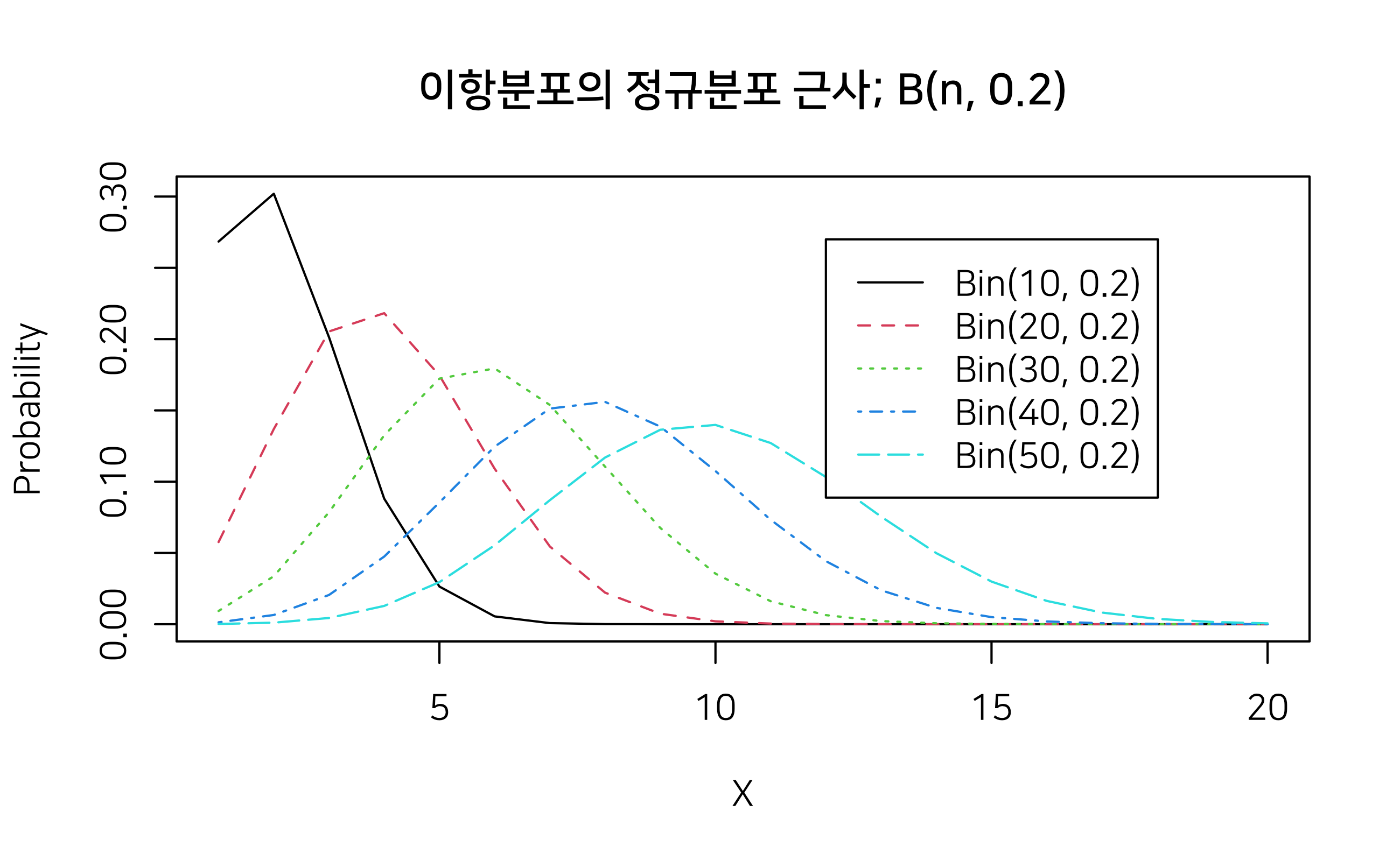
이항분포의 정규분포 근사

이항분포 B(n,p)에서 p값에 관계없이 n값이 충분히 커지면 이 분포는 정규분포에 근사하게 된다. 이것을 그래프로 그려 정규분포로 근사하는 것을 추적해 보았다. p=0.2이고 n=10, 20, 30, 40, 50인 이항분포를 한 좌표에 그려 보았다.

R Script

par(family = "NanumSquare")
plot(dbinom(1:20, 10, 0.2), type = "l", 
     main = "이항분포의 정규분포 근사; B(n, 0.2)", 
     xlab = "X", ylab = "Probability")

lines(dbinom(1:20, 20, 0.2), lty = 2, col = 2)
lines(dbinom(1:20, 30, 0.2), lty = 3, col = 3)
lines(dbinom(1:20, 40, 0.2), lty = 4, col = 4)
lines(dbinom(1:20, 50, 0.2), lty = 5, col = 5)

legend(12, 0.27, legend = c("Bin(10, 0.2)","Bin(20, 0.2)","Bin(30, 0.2)",
                            "Bin(40, 0.2)","Bin(50, 0.2)"),
       lty = 1:5, col = 1:5)

Comment on this article Share:

Citation

For attribution, please cite this work as

유충현 (2005, July 6). Dataholic: 이항분포의 정규분포 근사. Retrieved from https://choonghyunryu.github.io/posts/2005-07-06-binomial/

BibTeX citation

@misc{유충현2005이항분포의,
  author = {유충현, },
  title = {Dataholic: 이항분포의 정규분포 근사},
  url = {https://choonghyunryu.github.io/posts/2005-07-06-binomial/},
  year = {2005}
}