들어가기
배경
Machine Learning 기법을 이용해서 Documents Taxonomy를 수행하기 위한 Prototyping을 목적으로 한다.
분석 방법은 text2vec 패키지로 text를 vector 구조로 변환한 다음, Lasso and Elastic-Net Regularized Generalized Linear Models을 지원하는 glmnet 패키지를 이용해서 모델을 생성한다.
데이터 준비
그림과 같은 대통령기록연구실 홈페이지http://www.pa.go.kr/research/contents/speech/index.jsp 에는 역대 퇴임 대통령들의 연설문을 제공하고 있다.
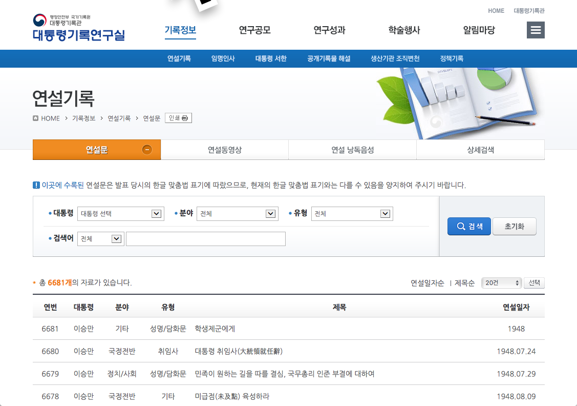
Figure 1: 대통령기록연구실 홈페이지
역대 대통령별로 연설문의 차이가 있는지 살펴보기 위해서 R로 Crawling 프로그램을 작성하여 이 홈페이지에서 김대중, 노무현, 이명박 전 대통령의 연설문 수집하였다.
이 leture에서는 김대중, 노무현, 이명박 전 대통령의 연설문만으로 모델을 생성하여, 연설문이 어느 전직 대통령이 연설한 것인지를 예측하는 방법으로 Documents Taxonomy 방법을 제시한다.
데이터 구조
수집한 데이터는 R 데이터 프레임 객체로 만들었으며, “data/speech.rda” 파일에 저장하였으며 변수는 다음과 같다.
- id
- 연설문(문서) 아이디
- president
- 연설 대통령
- category
- 연설문 분야
- type
- 연설문 유형
- title
- 연설문 제목
- data
- 연설 일자
- doc
- 연설문 내용
시작하기
패키지 로딩
데이터 로딩
“data/speech.rda” 파일로부터 데이터를 읽어 speech 데이퍼 프레임을 가져온다.
load("speech.rda")
Preparation data
data.table 객체 생성
데이터의 조작 속도의 개선을 위해서 data.frame 객체를 data.table 객체로 변환해주었다. 적은 양의 데이터는 data.frame 객체로 분석해도 상관 없지만, 일정 규모의 데이터 사이즈는 data.table 객체로 변환하여 분석하는 것이 바람직하다.
모델링을 위한 데이터셋 분리
연산 속도의 개선을 위해서 데이터 프레임 객체를 데이터 테이블 객체로 변환한다. 그리고 변환한 객체를 traing set과 test ste으로 분리한다.
random simple sampling을 수행하여 원 데이터를 traing : test = 70% : 30%로 분리를 수행한다.
Vectorization
모델링을 위해서 documents 데이터를 vector로 변환해야 한다. 이 경우 엄청난 데이터의 증가가 필연적으로 따라온다. 그래서 연산 속도의 개선을 위해서 vectorization 구조로 연산을 해야하기 때문에 Vectorization 연산을 수행하기 위한 구조로 변환해야 한다.
documents를 vector로 변환하는 tokenizer는 RMeCab 패키지를 이용해서 명사로 정의했다. 그러나 Mac 환경에서는 정상적으로 수행되었으나, 분석서버인 Centos Linux 환경에서는 에러가 발생하였다. 그래서 tokenizer는 명사가 아닌 words로 정의하였다. 이 경우에는 term의 개수가 증가하기 때문에 상대적으로 vector의 원소 개수가 증가하게된다.
또한 word2vec 패키지의 함수들은 parallel processing을 지원하므로, parallel 처리를 위한 multicores 사용을 지원하는 doMC, doParallel 패키지의 사용이 필요하다. 본 예제에서는 doMC 패키지를 사용한다.
noun_tokenizer <- function(docs, pos = c("NNG", "NNP")) {
  docs %>% lapply(function(x) {
    morpheme <- RMeCabC(x)
    morpheme <- unlist(morpheme[
      which(sapply(morpheme, names) %in% pos)])
    morpheme[nchar(morpheme) > 0]
  })
}

# not used
token_fun <- noun_tokenizer

token_fun <- tokenizers::tokenize_words

# parallel cores
nc <- parallel::detectCores()
registerDoMC(cores = nc)

it_train <- itoken_parallel(train$doc,
                   tokenizer = token_fun,
                   ids = train$id,
                   progressbar = FALSE)

it_test <- itoken_parallel(test$doc,
                  tokenizer = token_fun,
                  ids = test$id,
                  progressbar = FALSE)
모델 적합하기
Vocabulary 기반 모델링
Vocabulary 생성
vocabulary는 documents로부터 생성된 terms의 집합이다. 여기서는 tokenizer를 words로 정의했기 때문에 띄어쓰기 단위의 단어 집합으로 vocabulary가 생성된다.
몇몇 데이터를 조회해보면 term별로 frequency와 document frequency가 도출되었음을 알 수 있다.
vocab <- create_vocabulary(it_train)

tail(vocab, n = 10) %>%
  knitr::kable(., row.names = FALSE, format.args = list(big.mark = ","))
| term | term_count | doc_count |
|---|---|---|
| 한 | 3,846 | 1,129 |
| 그리고 | 4,136 | 1,226 |
| 이 | 4,991 | 1,216 |
| 있는 | 4,994 | 1,240 |
| 합니다 | 5,084 | 1,098 |
| 여러분 | 5,548 | 1,386 |
| 우리 | 7,395 | 1,444 |
| 수 | 8,449 | 1,381 |
| 것입니다 | 8,897 | 1,430 |
| 있습니다 | 11,950 | 1,527 |
Document Term Matrix 생성하기
documents taxonomy 분류 모델을 수행하는 데이터셋은 DTM(Document Term Matrix) 구조여야 한다. 그래서 vocabulary를 DTM으로 변환하는 작업을 수행한다.
vectorizer <-  vocab_vectorizer(vocab)

dtm_train <- create_dtm(it_train, vectorizer)
dim(dtm_train)
[1] 1685 127049dtm_test <- create_dtm(it_test, vectorizer)
dim(dtm_test)
[1] 723 127049모델 생성
모든 terms을 모델의 독립변수로 사용하려 하기 때문에, terms의 개수가 독립변수의 개수와 같게 된다. 이 경우에는 over-fitting의 이슈가 발생하므로 이를 해경하기 위해서 over-fitting을 방지해주는 LASSO 모델을 사용하기로 한다. 또한 target 변수가 binary가 아닌 3개의 class이기 때문에 family 함수는 “multinomial”을 지정한다. 즉, multinomial logistic regression의 알고리즘에 기반한 LASSO 모델을 만든다.
LASSO 모델을 생성하기 위해서는 cv.glmnet() 함수에서 penalty값인 alpha의 값을 1로 지정해야 LASSO Generalized Linear Model로 모델이 만들어진다. alpha의 값이 0이면 Ridge Generalized Linear Model, 0.5이면 Elastic Net Regularized Generalized Linear Model이 생성된다.
type.measure은 cross-validation을 위한 loss값 계산에 사용하는 측도를 지원한다. 일반적으로 binomial family 함수의 경우에는 type.measure 인수를 AUC(Area Under Curve)인 “auc”를 사용하지만, multinomial family 함수의 경우에는 이를 사용할 수 없기 때문에 여기서는 “deviance”를 사용하였다. 이 값이 기본값이다.
그리고 k-folds cross-validation의 k의 값은 10으로 지정하여, 10-fold cross-validation을 수행하여 over-fitting 또한 방지하도록 한다.
NFOLDS <- 10

classifier <- cv.glmnet(x = dtm_train, y = train$president,
                        family = 'multinomial',
                        alpha = 1,
                        type.measure = "deviance",
                        nfolds = NFOLDS,
                        thresh = 0.001,
                        maxit = 1000,
                        parallel = TRUE)
모델의 검증
test 데이터로 검증한 결과 Accuracy가 0.9378로 비교적 높게 나타났다.
pred_voca <- predict(classifier, dtm_test, type = 'response')[, , 1]
president_voca <- apply(pred_voca, 1,
                        function(x) colnames(pred_voca)[which(max(x) == x)])

cmat_voca <- caret::confusionMatrix(factor(president_voca), factor(test$president))
cmat_voca
Confusion Matrix and Statistics

          Reference
Prediction 김대중 노무현 이명박
    김대중    226      3      3
    노무현     16    220     10
    이명박      2      8    235

Overall Statistics

               Accuracy : 0.9419
                 95% CI : (0.9223, 0.9578)
    No Information Rate : 0.343
    P-Value [Acc > NIR] : < 2e-16

                  Kappa : 0.9129

 Mcnemar's Test P-Value : 0.02536

Statistics by Class:

                     Class: 김대중 Class: 노무현 Class: 이명박
Sensitivity                 0.9262        0.9524        0.9476
Specificity                 0.9875        0.9472        0.9789
Pos Pred Value              0.9741        0.8943        0.9592
Neg Pred Value              0.9633        0.9769        0.9728
Prevalence                  0.3375        0.3195        0.3430
Detection Rate              0.3126        0.3043        0.3250
Detection Prevalence        0.3209        0.3402        0.3389
Balanced Accuracy           0.9569        0.9498        0.9633
N-Grams 기반 모델링
N-grams은 N개의 연속된 terms의 조합을 terms로 간주하여 vocabulary를 생성하고 이 데이터 기반으로 모델을 생성한다. 파편화된 terms이 아니기 때문에 일반적인 vocabulary를 이용한 TA보다는 좀 더 정확하게 문맥을 파악할 수 있는 장점이 있다.
Vocabulary 생성
N-grams vocabulary는 create_vocabulary() 함수의 ngram 인수를 이용해서 생성한다. 여기서는 N의 값이 2인 2-grams 즉, bigram vocabulary를 생성한다.
vocab_bigram <- create_vocabulary(it_train, ngram = c(1L, 2L))

dim(vocab_bigram)
[1] 764734 3head(vocab_bigram, n = 10) %>%
knitr::kable(., row.names = FALSE, format.args = list(big.mark = ","))
| term | term_count | doc_count |
|---|---|---|
| 0.15 | 1 | 1 |
| 0.15_수준으로 | 1 | 1 |
| 0.1_를 | 1 | 1 |
| 0.1_미만의 | 1 | 1 |
| 0.230 | 1 | 1 |
| 0.230_입니다 | 1 | 1 |
| 0.291 | 1 | 1 |
| 0.291_에서 | 1 | 1 |
| 0.301 | 1 | 1 |
| 0.301_에 | 1 | 1 |
Prune Vocabulary
Documents의 개수가 증가하거나 Documents의 길이가 증가하면, Vocabulary의 규모도 증가한다. 이것은 모델을 생성하는데 많은 컴퓨팅 리소스를 소모해서 속도가 느려지게 된다. 그래서 모델에 영향을 덜 줄 수 있는 terms를 제거하는 작업이 필요하다.
prune_vocabulary() 함수는 Vocabulary에 포함된 terms를 제거하는 작업 수행해 준다. 여기서는 term_count_min 인수를 이용해서 term frequency가 10 미만이고, doc_proportion_max 인수를 이용해서 term을 포함해야하는 문서의 최대 비율이 0.5보다 큰 term을 제거하였다.
vocab_bigram <- vocab_bigram %>%
  prune_vocabulary(term_count_min = 10,
                   doc_proportion_max = 0.5)
dim(vocab_bigram)
[1] 18781 3Documents Term Matrix 생성
vectorizer_bigram <- vocab_vectorizer(vocab_bigram)

dtm_train_bigram <- create_dtm(it_train, vectorizer_bigram)
dim(dtm_train_bigram)
[1] 1685 18781dtm_test_bigram <- create_dtm(it_test, vectorizer_bigram)
dim(dtm_test_bigram)
[1] 723 18781모델 생성
classifier <- cv.glmnet(x = dtm_train_bigram, y = train$president,
                        family = 'multinomial',
                        type.measure = "deviance",
                        alpha = 1,
                        nfolds = NFOLDS,
                        parallel = TRUE)
모델 검증
vocabulary를 가지지기했음에도 불구하고, 전체 vocabulary를 사용한 모델보다 성능이 좋아졌다.
pred_bigram <- predict(classifier, dtm_test_bigram, type = 'response')[, , 1]

president_bigram <- apply(pred_bigram, 1,
                          function(x) colnames(pred_bigram)[which(max(x) == x)])

cmat_bigram <- confusionMatrix(factor(president_bigram), factor(test$president))
cmat_bigram
Confusion Matrix and Statistics

          Reference
Prediction 김대중 노무현 이명박
    김대중    232      2      7
    노무현     10    223     11
    이명박      2      6    230

Overall Statistics

               Accuracy : 0.9474
                 95% CI : (0.9286, 0.9625)
    No Information Rate : 0.343
    P-Value [Acc > NIR] : < 2e-16

                  Kappa : 0.9212

 Mcnemar's Test P-Value : 0.02248

Statistics by Class:

                     Class: 김대중 Class: 노무현 Class: 이명박
Sensitivity                 0.9508        0.9654        0.9274
Specificity                 0.9812        0.9573        0.9832
Pos Pred Value              0.9627        0.9139        0.9664
Neg Pred Value              0.9751        0.9833        0.9629
Prevalence                  0.3375        0.3195        0.3430
Detection Rate              0.3209        0.3084        0.3181
Detection Prevalence        0.3333        0.3375        0.3292
Balanced Accuracy           0.9660        0.9613        0.9553
Feature hashing 기반의 모델
Feature hashing은 Yahoo에서 개발한 기법으로 변수에 해시함수를 적용하고 이를 인덱스로 사용하는 기법이다. 이 방법을 적용하면 vecterization의 수행속도가 빨라지고, 연산 과정에서의 메로리 공간도 절약된다고 한다.
Hash Vectorize 정의
hash_vectorizer() 함수로 Feature hashing 적용한다.
vectorizer_hash <- hash_vectorizer(hash_size = 2 ^ 14, ngram = c(1L, 2L))
Document Term Matrix 생성
dtm_train_hash <- create_dtm(it_train, vectorizer_hash)
dtm_test_hash <- create_dtm(it_test, vectorizer_hash)
모델 생성
classifier <- cv.glmnet(x = dtm_train_hash, y = train$president,
                        family = 'multinomial',
                        type.multinomial = "grouped",
                        nfolds = NFOLDS,
                        thresh = 1e-3,
                        maxit = 1e3,
                        parallel = TRUE)
모델 검증
모델의 성능은 다른 기법보다는 낮아졌지만, 대용량의 데이터를 분석할 경우에는 속도의 개선을 위해서 사용해봄직 하다.
pred_hash <- predict(classifier, dtm_test_hash, type = 'response')[, , 1]

president_hash <- apply(pred_hash, 1,
                        function(x) colnames(pred_hash)[which(max(x) == x)])

cmat_hash <- confusionMatrix(factor(president_hash), factor(test$president))
cmat_hash
Confusion Matrix and Statistics

          Reference
Prediction 김대중 노무현 이명박
    김대중    222      5      2
    노무현     17    215      9
    이명박      5     11    237

Overall Statistics

               Accuracy : 0.9322
                 95% CI : (0.9114, 0.9494)
    No Information Rate : 0.343
    P-Value [Acc > NIR] : < 2e-16

                  Kappa : 0.8983

 Mcnemar's Test P-Value : 0.04537

Statistics by Class:

                     Class: 김대중 Class: 노무현 Class: 이명박
Sensitivity                 0.9098        0.9307        0.9556
Specificity                 0.9854        0.9472        0.9663
Pos Pred Value              0.9694        0.8921        0.9368
Neg Pred Value              0.9555        0.9668        0.9766
Prevalence                  0.3375        0.3195        0.3430
Detection Rate              0.3071        0.2974        0.3278
Detection Prevalence        0.3167        0.3333        0.3499
Balanced Accuracy           0.9476        0.9389        0.9610
TF-IDF 기반의 모델
대통령 연설문에서는 대부분 “존경하는 국민 여러분”으로 시작할 것이다. 그러므로 “존경하는”이라는 term은 모든 연설문에 포함되기 때문에 term frequency와 document term frequency가 상당히 클 것이다. 그러나 이 term으로 세명의 전직 대통령의 연설문을 구분하기 어렵다. 세명의 전직 대통령이 즐겨 사용하는 단어이기 때문이다. 즉, term frequency와 document term frequency가 상당히 큰 terms은 모델 개발에 의미가 없는 terms인 것이다.
TF-IDF는 단일문서, 혹은 소수의 문서에서 의미가 있는 terms의 가중치를 높이고 대부분의 문서에서 발현하는 terms의 가중치를 줄이는 용도로 만들어진 측도다. 그러므로 DTM에 TF-IDF 변환을 수행하면 모델의 성능이 개선된다.
Text Anaytics에서는 documents의 길이의 차이가 있으면, 상대적으로 짧거나 긴 documents에서 발현하는 terms들로 인해서 frequency scale에 왜곡이 있을 수 있다. 이 경우에는 표준화를 수행해야 한다. 그런데 TF-IDF 변환은 자동으로 표준화가 되기 때문에 표준화의 잇점이 있다. 만약 표준화를 수행하려면, normalize() 함수를 사용하면 된다.
DTM의 TF-IDF 변환
TfIdf class와 fit_transform() 함수를 이용해서 DTM에 TF-IDF 변환을 수행한다.
tfidf <- TfIdf$new()

dtm_train_tfidf <- fit_transform(dtm_train, tfidf)
dtm_test_tfidf <- fit_transform(dtm_test, tfidf)
모델 생성
classifier <- cv.glmnet(x = dtm_train_tfidf, y = train$president,
                        family = 'multinomial',
                        nfolds = NFOLDS,
                        thresh = 1e-3,
                        maxit = 1e3,
                        parallel = TRUE)
모델의 검증
TF-IDF 변환된 데이터로 생성한 모델의 성능이 상대적으로 높다.
pred_tfidf <- predict(classifier, dtm_test_tfidf, type = 'response')[, , 1]

president_tfidf <- apply(pred_tfidf, 1,
                         function(x) colnames(pred_tfidf)
                         [which(max(x) == x)])

cmat_tfidf <- confusionMatrix(factor(president_tfidf), factor(test$president))
cmat_tfidf
Confusion Matrix and Statistics

          Reference
Prediction 김대중 노무현 이명박
    김대중    236      5      3
    노무현      7    218      4
    이명박      1      8    241

Overall Statistics

               Accuracy : 0.9613
                 95% CI : (0.9445, 0.9741)
    No Information Rate : 0.343
    P-Value [Acc > NIR] : <2e-16

                  Kappa : 0.9419

 Mcnemar's Test P-Value : 0.4459

Statistics by Class:

                     Class: 김대중 Class: 노무현 Class: 이명박
Sensitivity                 0.9672        0.9437        0.9718
Specificity                 0.9833        0.9776        0.9811
Pos Pred Value              0.9672        0.9520        0.9640
Neg Pred Value              0.9833        0.9737        0.9852
Prevalence                  0.3375        0.3195        0.3430
Detection Rate              0.3264        0.3015        0.3333
Detection Prevalence        0.3375        0.3167        0.3458
Balanced Accuracy           0.9753        0.9607        0.9764
모델 성능의 비교
모델의 성능은 TF-IDF > Bigram > Vocabulary > Feature Hashing의 순서로 나타난다.
그러므로 성능을 높이기 위해서는 TF-IDF 방법을 사용하는 것이 좋으며, 대용량의 데이터 분석에서는 적은 성능 감소와 수행 속도의 개선을 가져오는 Feature Hashing 기법을 사용하면 될 것이다. 이 경우에는 Purne Vocabulary 전처리도 필요할 것이다.
accuracy <- rbind(cmat_voca$overall, cmat_bigram$overall,
                  cmat_hash$overall, cmat_tfidf$overall) %>%
  round(3)

data.frame(Method = c("Vocabulary", "Bigram", "FeatueHash", "TF-IDF"),
           accuracy) %>%
  arrange(desc(Accuracy)) %>%
  knitr::kable()
| Method | Accuracy | Kappa | AccuracyLower | AccuracyUpper | AccuracyNull | AccuracyPValue | McnemarPValue |
|---|---|---|---|---|---|---|---|
| TF-IDF | 0.961 | 0.942 | 0.945 | 0.974 | 0.343 | 0 | 0.446 |
| Bigram | 0.947 | 0.921 | 0.929 | 0.963 | 0.343 | 0 | 0.022 |
| Vocabulary | 0.942 | 0.913 | 0.922 | 0.958 | 0.343 | 0 | 0.025 |
| FeatueHash | 0.932 | 0.898 | 0.911 | 0.949 | 0.343 | 0 | 0.045 |
Reference
본 분석 사례는 Vectorization(‘http://text2vec.org/vectorization.html’)을 참고하였다.