dlookr - 데이터 변환

이 문서는 dlookr 기능 중에서 데이터 변환 기능을 소개한다. 여러분은 dlookr에서 제공하는 함수로 데이터 프레임과 데이터 프레임을 상속한 tbl_df 데이터의 데이터 변환을 수행하는 방법을 일힐 수 있을 것이다.

일러두기

분석을 위한 데이터를 획득한 후에는 다음을 수행해야 한다.:

• 데이터의 품질을 진단한다.
  • 만약 데이터 품질의 문제를 발견한다면,
  • 문제의 데이터를 보완하거나 경우에 따라서는 재획득을 수행햐야 한다.
• 데이터를 이해하기 위한 탐색을 수행하여, 분석의 전개 방향에 대한 시나리오를 수립한다.
• 분석에 효과적인 변수를 파생하거나 변수의 변환을 수행한다.

dlookr 패키지는 다음의 과정을 빠르고 쉽게 수행하도록 도움을 준다.

• 데이터의 진단을 수행하거나 데이터 품질 진단 리포트를 자동으로 생성한다.
• 다양한 방법으로 데이터를 탐색하고 EDA(탐색적 데이터 분석) 보고서를 생성한다.
• 결측치와 이상치를 대체하고, 치우친 데이터를 보정하며, 연속형 변수를 비닝(binning)하여 범주형 변수로 만든다. 그리고 이를 지원하는 자동화된 리포트를 생성한다.

이 문서는 dlookr 기능 중에서 데이터 변환 기능을 소개한다. 여러분은 dlookr에서 제공하는 함수로 데이터 프레임과 데이터 프레임을 상속한 tbl_df 데이터의 데이터 변환을 수행하는 방법을 일힐 수 있을 것이다.

dlookr 패키지는 dplyr 패키지와 함께 사용하면 시너지가 증가된다. 특히 데이터 변환에서 tidyverse 패키지 그룹의 효율성을 높여준다.

데이터

dlookr 패키지로 EDA를 수행하는 기초적인 사용 방법을 설명하기 위해서 Carseats를 사용한다. ISLR 패키지의 Carseats는 400개의 매장에서 아동용 카시트를 판매하는 시뮬레이션 데이터다. 이 데이터는 판매량을 예측하는 목적으로 생성한 데이터 프레임이다.

library(ISLR)
str(Carseats)

'data.frame':   400 obs. of  11 variables:
 $ Sales      : num  9.5 11.22 10.06 7.4 4.15 ...
 $ CompPrice  : num  138 111 113 117 141 124 115 136 132 132 ...
 $ Income     : num  73 48 35 100 64 113 105 81 110 113 ...
 $ Advertising: num  11 16 10 4 3 13 0 15 0 0 ...
 $ Population : num  276 260 269 466 340 501 45 425 108 131 ...
 $ Price      : num  120 83 80 97 128 72 108 120 124 124 ...
 $ ShelveLoc  : Factor w/ 3 levels "Bad","Good","Medium": 1 2 3 3 1 1 3 2 3 3 ...
 $ Age        : num  42 65 59 55 38 78 71 67 76 76 ...
 $ Education  : num  17 10 12 14 13 16 15 10 10 17 ...
 $ Urban      : Factor w/ 2 levels "No","Yes": 2 2 2 2 2 1 2 2 1 1 ...
 $ US         : Factor w/ 2 levels "No","Yes": 2 2 2 2 1 2 1 2 1 2 ...

개별 변수들의 의미는 다음과 같다. (ISLR::Carseats Man page 참고)

• Sales
  • 지역의 단위 판매량 (단위: 천개)
• CompPrice
  • 지역의 경쟁 업체가 부과하는 가격
• Income
  • 지역 공동체 수입 수준 (단위: 천달러)
• Advertising
  • 회사의 지역에 대한 광고 예산 (단위: 천달러)
• Population
  • 지역의 인구 규모 (단위: 천명)
• Price
  • 지역의 자동차 좌석 요금
• ShelveLoc
  • 각 사이트에서 자동차 좌석의 선반 위치의 품질을 나타내는 수준. “Bad”, “Good”, “Medium”.
• Age
  • 각 지역의 평균 연령
• Education
  • 각 지역의 교육 수준
• Urban
  • 점포의 도시 또는 농촌 소재 여부. Yes는 도시, No는 농촌.
• US
  • 점포의 미국 소재 여부. Yes는 미국 소재, No는 미국 외 소재.

데이터 분석을 수행할 때, 결측치가 포함된 데이터를 자주 접한다. 그러나 Carseats는 결측치가 없은 완전한 데이터다. 그래서 다음과 같이 결측치를 생성하였다. 그리고 carseats라는 이름의 데이터 프레임 객체를 생성한다.

carseats <- ISLR::Carseats

set.seed(123)
carseats[sample(seq(NROW(carseats)), 20), "Income"] <- NA

set.seed(456)
carseats[sample(seq(NROW(carseats)), 10), "Urban"] <- NA

데이터 변환

dlookr은 결측치와 이상치의 대체, 치우친 데이터를 보정해준다. 또한 연속형 변수를 범주형 변수로 비닝하는 것을 도와준다.

다음은 dlookr이 제공하는 데이터 변환 함수와 함수의 기능 목록이다.:

• find_na()는 결측치가 포함된 변수를 찾아주고, imputate_na()는 결측치를 대체한다.
• find_outliers()는 이상치가 포함된 변수를 찾아주고, imputate_outlier()는 이상치를 대체한다.
• summary.imputation()와 plot.imputation()는 대체된 변수의 정보를 보혀주고 시각화를 제공한다.
• find_skewness()는 치우친 데이터의 변수를 찾아주고, transform()는 치우친 데이터의 보정을 수행한다.
• 또한 transform()는 수치형 변수의 표준화를 수행한다.
• summary.transform()와 plot.transform()는 변환된 변수의 정보를 보혀주고 시각화를 제공한다.
• binning()와 binning_by()는 수치 데이터를 비닝하여 범주형 데이터로 변환한다.
• print.bins()와 summary.bins()는 비닝 결과를 보여주고 요약해 준다.
• plot.bins()와 plot.optimal_bins()는 비닝 결과의 시각화를 제공한다.
• transformation_report()는 데이터 변환을 수행한 후 그 결과를 보고서로 만들어 준다.

결측치의 대체

imputate_na()을 이용한 결측치의 대체

imputate_na()는 변수에 포함된 결측치를 대체한다. 결측치가 포함된 예측변수(predictor)는 수치형 변수와 범주형 변수 모두 지원하며, 다음과 같은 method를 지원한다.

• predictor가 수치형 변수일 경우
  • “mean” : 산술평균으로 대체
  • “median” : 중위수로 대체
  • “mode” : 최빈수로 대체
  • “knn” : K-nearest neighbors를 이용한 대체
    • target 변수를 지정해야 함
  • “rpart” : Recursive Partitioning and Regression Trees를 이용한 대체
    • target 변수를 지정해야 함
      
  • “mice” : Multivariate Imputation by Chained Equations를 이용한 대체
    • target 변수를 지정해야 함
    • random seed를 지정해야 함
• predictor가 범주형 변수일 경우
  • “mode” : 최빈수로 대체
  • “rpart” : Recursive Partitioning and Regression Trees를 이용한 대체
    • target 변수를 지정해야 함
      
  • “mice” : Multivariate Imputation by Chained Equations를 이용한 대체
    • target 변수를 지정해야 함
      
    • random seed를 지정해야 함

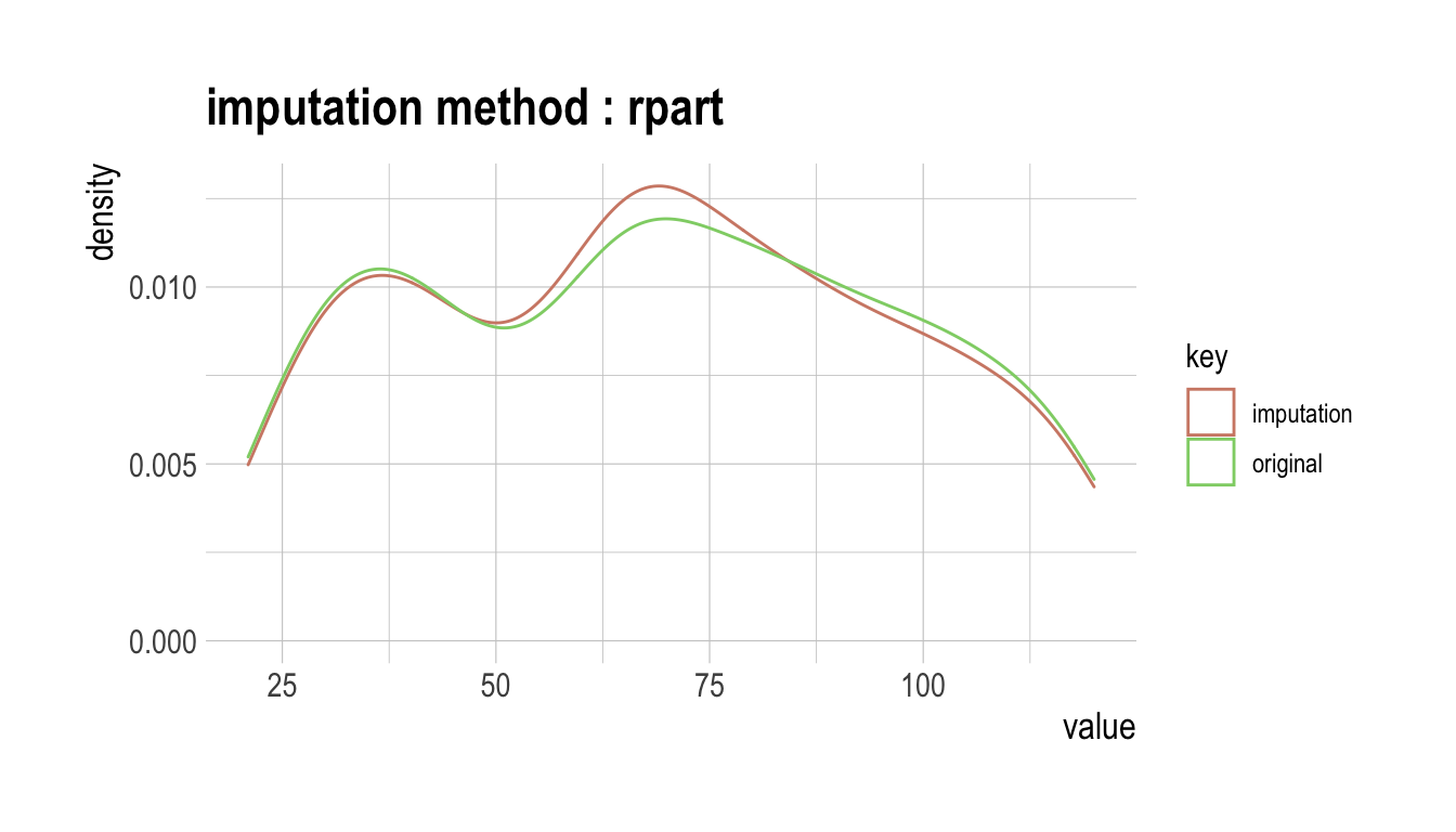
다음처럼 imputate_na()는 carseats의 수치형 변수인 Income를 “rpart” 방법으로 결측치를 대체한다. summary()는 결측치 대체 정보를 요약하고, plot()은 결측정보를 시각화한다.

income <- imputate_na(carseats, Income, US, method = "rpart")

# result of imputate
income

  [1]  73.00000  48.00000  35.00000 100.00000  64.00000 113.00000
  [7] 105.00000  81.00000 110.00000 113.00000  78.00000  94.00000
 [13]  35.00000  58.63636 117.00000  95.00000  32.00000  74.00000
 [19] 110.00000  76.00000  90.00000  29.00000  46.00000  31.00000
 [25] 119.00000  32.00000 115.00000 118.00000  74.00000  99.00000
 [31]  94.00000  58.00000  32.00000  38.00000  54.00000  84.00000
 [37]  76.00000  41.00000  73.00000  60.00000  98.00000  53.00000
 [43]  69.00000  42.00000  79.00000  63.00000  90.00000  98.00000
 [49]  52.00000  93.00000  32.00000  90.00000  40.00000  64.00000
 [55] 103.00000  81.00000  82.00000  91.00000  93.00000  71.00000
 [61] 102.00000  32.00000  45.00000  88.00000  67.00000  26.00000
 [67]  92.00000  61.00000  69.00000  59.00000  81.00000  51.00000
 [73]  45.00000  90.00000  68.00000 111.00000  87.00000  71.00000
 [79]  48.00000  67.00000 100.00000  72.00000  83.00000  36.00000
 [85]  25.00000 103.00000  84.00000  67.00000  42.00000  56.07143
 [91]  67.14286  46.00000 113.00000  30.00000  97.00000  25.00000
 [97]  42.00000  82.00000  77.00000  47.00000  69.00000  93.00000
[103]  22.00000  91.00000  96.00000 100.00000  33.00000 107.00000
[109]  79.00000  65.00000  62.00000 118.00000  99.00000  29.00000
[115]  87.00000  35.00000  75.00000  75.34722  88.00000  94.00000
[121] 105.00000  89.00000 100.00000 103.00000 113.00000  78.00000
[127]  68.00000  48.00000 100.00000 120.00000  84.00000  69.00000
[133]  87.00000  98.00000  31.00000  94.00000  68.81481  42.00000
[139] 103.00000  62.00000  60.00000  42.00000  84.00000  88.00000
[145]  68.00000  63.00000  83.00000  54.00000 119.00000 120.00000
[151]  84.00000  58.00000  67.77778  36.00000  69.00000  72.00000
[157]  34.00000  58.00000  90.00000  60.00000  28.00000  21.00000
[163]  74.00000  64.00000  64.00000  58.00000  67.00000  73.00000
[169]  89.00000  41.00000  39.00000 106.00000 102.00000  91.00000
[175]  24.00000  89.00000 107.00000  72.00000  89.86364  25.00000
[181] 112.00000  83.00000  60.00000  74.00000  33.00000 100.00000
[187]  51.00000  32.00000  37.00000 117.00000  37.00000  42.00000
[193]  26.00000  70.00000  56.07143  93.00000  65.50000  61.00000
[199]  80.00000  88.00000  92.00000  83.00000  78.00000  82.00000
[205]  80.00000  22.00000  67.00000 105.00000  54.00000  21.00000
[211]  41.00000 118.00000  69.00000  84.00000 115.00000  83.00000
[217]  33.00000  44.00000  61.00000  79.00000 120.00000  44.00000
[223] 119.00000  45.00000  82.00000  25.00000  33.00000  64.00000
[229]  67.50000 104.00000  60.00000  69.00000  80.00000  76.00000
[235]  62.00000  32.00000  34.00000  28.00000  24.00000 105.00000
[241]  80.00000  63.00000  46.00000  68.81481  30.00000  43.00000
[247]  56.00000 114.00000  52.00000  67.00000 105.00000 111.00000
[253]  97.00000  24.00000 104.00000  55.55556  40.00000  62.00000
[259]  38.00000  36.00000 117.00000  42.00000  77.00000  26.00000
[265]  29.00000  35.00000  93.00000  82.00000  57.00000  69.00000
[271]  26.00000  56.00000  33.00000 106.00000  93.00000 119.00000
[277]  69.00000  48.00000 113.00000  57.00000  86.00000  69.00000
[283]  96.00000 110.00000  46.00000  26.00000 118.00000  44.00000
[289]  40.00000  77.00000 111.00000  70.00000  66.00000  84.00000
[295]  76.00000  35.00000  44.00000  83.00000  75.34722  40.00000
[301]  78.00000  93.00000  77.00000  52.00000  98.00000  67.77778
[307]  32.00000  92.00000  80.00000 111.00000  65.00000  68.00000
[313] 117.00000  81.00000  33.00000  21.00000  36.00000  30.00000
[319]  72.00000  45.00000  70.00000  39.00000  50.00000 105.00000
[325]  65.00000  69.00000  30.00000  41.72727  66.00000  54.00000
[331]  59.00000  63.00000  33.00000  60.00000 117.00000  70.00000
[337]  35.00000  38.00000  24.00000  44.00000  29.00000 120.00000
[343] 102.00000  42.00000  80.00000  68.00000 107.00000  31.85714
[349] 102.00000  27.00000 101.00000 115.00000 103.00000  67.00000
[355]  68.81481 100.00000 109.00000  73.00000  96.00000  62.00000
[361]  86.00000  25.00000  55.00000  75.00000  21.00000  30.00000
[367]  56.00000 106.00000  22.00000 100.00000  41.00000  81.00000
[373]  50.00000  83.77778  47.00000  46.00000  60.00000  61.00000
[379]  88.00000 111.00000  64.00000  65.00000  28.00000 117.00000
[385]  37.00000  73.00000 116.00000  75.34722  89.00000  42.00000
[391]  75.00000  63.00000  42.00000  51.00000  58.00000 108.00000
[397]  23.00000  26.00000  47.50000  37.00000
attr(,"var_type")
[1] "numerical"
attr(,"method")
[1] "rpart"
attr(,"na_pos")
 [1]  14  90  91 118 137 153 179 195 197 229 244 256 299 306 328 348
[17] 355 374 388 399
attr(,"type")
[1] "missing values"
attr(,"message")
[1] "complete imputation"
attr(,"success")
[1] TRUE
attr(,"class")
[1] "imputation" "numeric"   

# summary of imputate
summary(income)

* Impute missing values based on Recursive Partitioning and Regression Trees
 - method : rpart

* Information of Imputation (before vs after)
             Original   Imputation
n        380.00000000 400.00000000
na        20.00000000   0.00000000
mean      69.32105263  69.07811282
sd        28.06686473  27.53886441
se_mean    1.43979978   1.37694322
IQR       48.00000000  45.50000000
skewness   0.03601821   0.05313579
kurtosis  -1.10286001  -1.04030028
p00       21.00000000  21.00000000
p01       21.79000000  21.99000000
p05       26.00000000  26.00000000
p10       31.90000000  32.00000000
p20       40.00000000  41.00000000
p25       44.00000000  44.75000000
p30       50.00000000  51.00000000
p40       62.00000000  62.00000000
p50       69.00000000  69.00000000
p60       78.00000000  77.00000000
p70       87.30000000  84.60000000
p75       92.00000000  90.25000000
p80       98.00000000  96.00000000
p90      108.10000000 107.00000000
p95      115.05000000 115.00000000
p99      119.21000000 119.01000000
p100     120.00000000 120.00000000

# viz of imputate
plot(income)

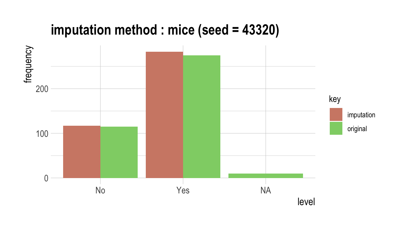
다음은 범주형 변수인 urban을 “mice” 방법으로 결측치를 대체한다. summary()는 결측치 대체 정보를 요약하고, plot()은 결측정보를 시각화한다.

library(mice)

urban <- imputate_na(carseats, Urban, US, method = "mice")

 iter imp variable
  1   1  Income  Urban
  1   2  Income  Urban
  1   3  Income  Urban
  1   4  Income  Urban
  1   5  Income  Urban
  2   1  Income  Urban
  2   2  Income  Urban
  2   3  Income  Urban
  2   4  Income  Urban
  2   5  Income  Urban
  3   1  Income  Urban
  3   2  Income  Urban
  3   3  Income  Urban
  3   4  Income  Urban
  3   5  Income  Urban
  4   1  Income  Urban
  4   2  Income  Urban
  4   3  Income  Urban
  4   4  Income  Urban
  4   5  Income  Urban
  5   1  Income  Urban
  5   2  Income  Urban
  5   3  Income  Urban
  5   4  Income  Urban
  5   5  Income  Urban

# result of imputate
urban

  [1] Yes Yes Yes Yes Yes No  Yes Yes No  No  No  Yes Yes Yes Yes No 
 [17] Yes Yes No  Yes Yes No  Yes Yes Yes No  No  Yes Yes Yes Yes Yes
 [33] No  Yes Yes No  No  No  Yes No  No  Yes Yes Yes Yes Yes No  Yes
 [49] Yes Yes Yes Yes Yes Yes No  Yes Yes Yes Yes Yes Yes No  Yes Yes
 [65] No  No  Yes Yes Yes Yes Yes No  Yes No  No  No  Yes No  Yes Yes
 [81] Yes Yes Yes Yes No  No  Yes No  Yes Yes No  Yes Yes Yes Yes Yes
 [97] No  Yes No  No  No  Yes No  Yes Yes Yes No  Yes Yes No  Yes Yes
[113] Yes Yes Yes Yes No  Yes Yes Yes Yes Yes Yes No  Yes No  Yes Yes
[129] Yes No  Yes Yes Yes Yes Yes No  No  Yes Yes No  Yes Yes Yes Yes
[145] No  Yes Yes No  No  Yes No  No  No  No  No  Yes Yes No  Yes No 
[161] No  No  Yes No  No  Yes Yes Yes Yes Yes Yes Yes Yes Yes No  Yes
[177] No  Yes No  Yes Yes Yes Yes Yes No  Yes No  Yes Yes No  No  Yes
[193] No  Yes Yes Yes Yes Yes Yes Yes No  Yes No  Yes Yes Yes Yes No 
[209] Yes No  No  Yes Yes Yes Yes Yes Yes No  Yes Yes Yes Yes Yes Yes
[225] No  Yes Yes Yes No  No  No  No  Yes No  No  Yes Yes Yes Yes Yes
[241] Yes Yes No  Yes Yes No  Yes Yes Yes Yes Yes Yes Yes No  Yes Yes
[257] Yes Yes No  No  Yes Yes Yes Yes Yes Yes No  No  Yes Yes Yes Yes
[273] Yes Yes Yes Yes Yes Yes No  Yes Yes No  Yes No  No  Yes No  Yes
[289] No  Yes No  Yes Yes Yes Yes No  Yes Yes Yes No  Yes Yes Yes Yes
[305] Yes Yes Yes Yes Yes Yes Yes Yes Yes Yes Yes Yes Yes No  No  No 
[321] Yes Yes Yes Yes Yes Yes Yes Yes Yes Yes No  Yes Yes Yes Yes Yes
[337] Yes Yes Yes Yes Yes No  No  Yes No  Yes No  No  Yes No  No  No 
[353] Yes No  Yes Yes Yes Yes Yes Yes No  No  Yes Yes Yes No  No  Yes
[369] No  Yes Yes Yes No  Yes Yes Yes Yes No  Yes Yes Yes Yes Yes Yes
[385] Yes Yes Yes No  Yes Yes Yes Yes Yes No  Yes Yes No  Yes Yes Yes
attr(,"var_type")
[1] categorical
attr(,"method")
[1] mice
attr(,"na_pos")
 [1]  38  90 159 206 237 252 281 283 335 378
attr(,"seed")
[1] 43320
attr(,"type")
[1] missing values
attr(,"message")
[1] complete imputation
attr(,"success")
[1] TRUE
Levels: No Yes

# summary of imputate
summary(urban)

* Impute missing values based on Multivariate Imputation by Chained Equations
 - method : mice
 - random seed : 43320

* Information of Imputation (before vs after)
     original imputation original_percent imputation_percent
No        115        117            28.75              29.25
Yes       275        283            68.75              70.75
<NA>       10          0             2.50               0.00

# viz of imputate
plot(urban)

dplyr과의 협업

다음은 dplyr를 이용해서 이상치를 대체한 Income 변수를 US의 수준별로 산술평균을 구하는 예제다.

# The mean before and after the imputation of the Income variable
carseats %>%
  mutate(Income_imp = imputate_na(carseats, Income, US, method = "knn")) %>%
  group_by(US) %>%
  summarise(orig = mean(Income, na.rm = TRUE),
    imputation = mean(Income_imp))

# A tibble: 2 x 3
  US     orig imputation
  <fct> <dbl>      <dbl>
1 No     65.7       65.5
2 Yes    71.3       71.5

이상치의 대체

imputate_outlier()을 이용한 이상치의 대체

imputate_outlier()는 변수에 포함된 이상치를 대체한다. 이상치가 포함된 예측변수(predictor)는 수치형 변수만 지원하며, 다음과 같은 method를 지원한다.

• predictor가 수치형 변수일 경우
  • “mean” : 산술평균으로 대체
  • “median” : 중위수로 대체
  • “mode” : 최빈수로 대체
  • “capping” : 상위 이상치를 95/백분위수로 대체하고 하위 이상치를 5/백분위수로 대체

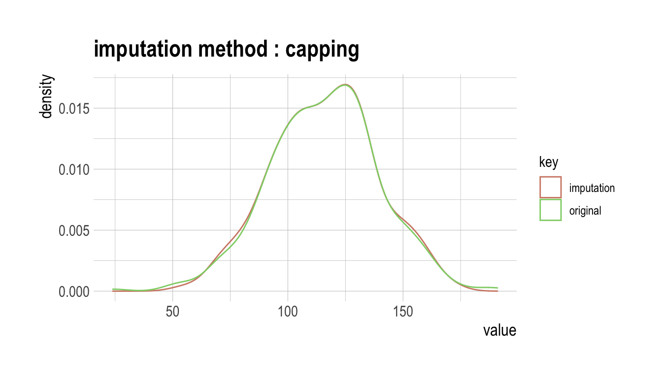
다음처럼 imputate_outlier()는 carseats의 수치형 변수인 Price를 “capping” 방법으로 이상치를 대체한다. summary()는 이상치 대체 정보를 요약하고, plot()은 결측정보를 시각화한다.

price <- imputate_outlier(carseats, Price, method = "capping")

# result of imputate
price

  [1] 120.00  83.00  80.00  97.00 128.00  72.00 108.00 120.00 124.00
 [10] 124.00 100.00  94.00 136.00  86.00 118.00 144.00 110.00 131.00
 [19]  68.00 121.00 131.00 109.00 138.00 109.00 113.00  82.00 131.00
 [28] 107.00  97.00 102.00  89.00 131.00 137.00 128.00 128.00  96.00
 [37] 100.00 110.00 102.00 138.00 126.00 124.00  77.00 134.00  95.00
 [46] 135.00  70.00 108.00  98.00 149.00 108.00 108.00 129.00 119.00
 [55] 144.00 154.00  84.00 117.00 103.00 114.00 123.00 107.00 133.00
 [64] 101.00 104.00 128.00  91.00 115.00 134.00  99.00  99.00 150.00
 [73] 116.00 104.00 136.00  92.00  70.00  89.00 145.00  90.00  79.00
 [82] 128.00 139.00  94.00 121.00 112.00 134.00 126.00 111.00 119.00
 [91] 103.00 107.00 125.00 104.00  84.00 148.00 132.00 129.00 127.00
[100] 107.00 106.00 118.00  97.00  96.00 138.00  97.00 139.00 108.00
[109] 103.00  90.00 116.00 151.00 125.00 127.00 106.00 129.00 128.00
[118] 119.00  99.00 128.00 131.00  87.00 108.00 155.00 120.00  77.00
[127] 133.00 116.00 126.00 147.00  77.00  94.00 136.00  97.00 131.00
[136] 120.00 120.00 118.00 109.00  94.00 129.00 131.00 104.00 159.00
[145] 123.00 117.00 131.00 119.00  97.00  87.00 114.00 103.00 128.00
[154] 150.00 110.00  69.00 157.00  90.00 112.00  70.00 111.00 160.00
[163] 149.00 106.00 141.00 155.05 137.00  93.00 117.00  77.00 118.00
[172]  55.00 110.00 128.00 155.05 122.00 154.00  94.00  81.00 116.00
[181] 149.00  91.00 140.00 102.00  97.00 107.00  86.00  96.00  90.00
[190] 104.00 101.00 173.00  93.00  96.00 128.00 112.00 133.00 138.00
[199] 128.00 126.00 146.00 134.00 130.00 157.00 124.00 132.00 160.00
[208]  97.00  64.00  90.00 123.00 120.00 105.00 139.00 107.00 144.00
[217] 144.00 111.00 120.00 116.00 124.00 107.00 145.00 125.00 141.00
[226]  82.00 122.00 101.00 163.00  72.00 114.00 122.00 105.00 120.00
[235] 129.00 132.00 108.00 135.00 133.00 118.00 121.00  94.00 135.00
[244] 110.00 100.00  88.00  90.00 151.00 101.00 117.00 156.00 132.00
[253] 117.00 122.00 129.00  81.00 144.00 112.00  81.00 100.00 101.00
[262] 118.00 132.00 115.00 159.00 129.00 112.00 112.00 105.00 166.00
[271]  89.00 110.00  63.00  86.00 119.00 132.00 130.00 125.00 151.00
[280] 158.00 145.00 105.00 154.00 117.00  96.00 131.00 113.00  72.00
[289]  97.00 156.00 103.00  89.00  74.00  89.00  99.00 137.00 123.00
[298] 104.00 130.00  96.00  99.00  87.00 110.00  99.00 134.00 132.00
[307] 133.00 120.00 126.00  80.00 166.00 132.00 135.00  54.00 129.00
[316] 171.00  72.00 136.00 130.00 129.00 152.00  98.00 139.00 103.00
[325] 150.00 104.00 122.00 104.00 111.00  89.00 112.00 134.00 104.00
[334] 147.00  83.00 110.00 143.00 102.00 101.00 126.00  91.00  93.00
[343] 118.00 121.00 126.00 149.00 125.00 112.00 107.00  96.00  91.00
[352] 105.00 122.00  92.00 145.00 146.00 164.00  72.00 118.00 130.00
[361] 114.00 104.00 110.00 108.00 131.00 162.00 134.00  77.00  79.00
[370] 122.00 119.00 126.00  98.00 116.00 118.00 124.00  92.00 125.00
[379] 119.00 107.00  89.00 151.00 121.00  68.00 112.00 132.00 160.00
[388] 115.00  78.00 107.00 111.00 124.00 130.00 120.00 139.00 128.00
[397] 120.00 159.00  95.00 120.00
attr(,"method")
[1] "capping"
attr(,"var_type")
[1] "numerical"
attr(,"outlier_pos")
[1]  43 126 166 175 368
attr(,"outliers")
[1]  24  49 191 185  53
attr(,"type")
[1] "outliers"
attr(,"message")
[1] "complete imputation"
attr(,"success")
[1] TRUE
attr(,"class")
[1] "imputation" "numeric"   

# summary of imputate
summary(price)

Impute outliers with capping

* Information of Imputation (before vs after)
            Original  Imputation
n        400.0000000 400.0000000
na         0.0000000   0.0000000
mean     115.7950000 115.8927500
sd        23.6766644  22.6109187
se_mean    1.1838332   1.1305459
IQR       31.0000000  31.0000000
skewness  -0.1252862  -0.0461621
kurtosis   0.4518850  -0.3030578
p00       24.0000000  54.0000000
p01       54.9900000  67.9600000
p05       77.0000000  77.0000000
p10       87.0000000  87.0000000
p20       96.8000000  96.8000000
p25      100.0000000 100.0000000
p30      104.0000000 104.0000000
p40      110.0000000 110.0000000
p50      117.0000000 117.0000000
p60      122.0000000 122.0000000
p70      128.3000000 128.3000000
p75      131.0000000 131.0000000
p80      134.0000000 134.0000000
p90      146.0000000 146.0000000
p95      155.0500000 155.0025000
p99      166.0500000 164.0200000
p100     191.0000000 173.0000000

# viz of imputate
plot(price)

dplyr과의 협업

다음은 dplyr를 이용해서 이상치를 대체한 Price 변수를 US의 수준별로 산술평균을 구하는 예제다.

# The mean before and after the imputation of the Price variable
carseats %>%
  mutate(Price_imp = imputate_outlier(carseats, Price, method = "capping")) %>%
  group_by(US) %>%
  summarise(orig = mean(Price, na.rm = TRUE),
    imputation = mean(Price_imp, na.rm = TRUE))

# A tibble: 2 x 3
  US     orig imputation
  <fct> <dbl>      <dbl>
1 No     114.       114.
2 Yes    117.       117.

표준화와 치우친 데이터의 보정

transform()의 기능

transform()는 변수를 변환한다. 수치형 변수만 지원하며, 다음과 같은 method를 제공한다.

• 표준화
  • “zscore” : z-score 변환. (x - mu) / sigma
  • “minmax” : minmax 변환. (x - min) / (max - min)
• 치우침 보정
  • “log” : log 변환. log(x)
  • “log+1” : log 변환. log(x + 1). 0을 포함한 값들이 많을 때 유용함.
  • “sqrt” : 제곱근 변환
  • “1/x” : 1 / x 변환
  • “x^2” : 제곱 변환
  • “x^3” : 세제곱 변환

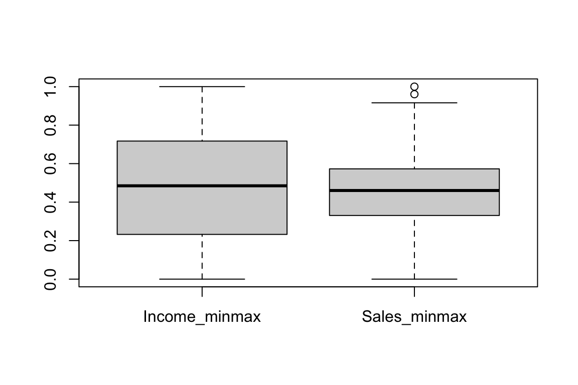
transform()을 이용한 표준화

표준화를 수행하는 method “zscore”와 “minmax”를 이용한다.

carseats %>% 
  mutate(Income_minmax = transform(carseats$Income, method = "minmax"),
    Sales_minmax = transform(carseats$Sales, method = "minmax")) %>% 
  select(Income_minmax, Sales_minmax) %>% 
  boxplot()

transform()을 이용한 치우친 데이터의 보정

find_skewness()는 치우친 데이터를 찾기 위해서 왜도를 구한다.

# find index of skewed variables
find_skewness(carseats)

[1] 4

# find names of skewed variables
find_skewness(carseats, index = FALSE)

[1] "Advertising"

# compute the skewness
find_skewness(carseats, value = TRUE)

      Sales   CompPrice      Income Advertising  Population 
      0.185      -0.043       0.036       0.637      -0.051 
      Price         Age   Education 
     -0.125      -0.077       0.044 

# compute the skewness & filtering with threshold
find_skewness(carseats, value = TRUE, thres = 0.1)

      Sales Advertising       Price 
      0.185       0.637      -0.125 

Advertising의 왜도가 0.637로 좌측으로 어느정도 기울어져 있어서 다음처럼 transformation()를 이용해서 “log” 방법으로 변환한다. summary()는 변환정보를 요약하고, plot()은 변환정보를 시각화한다.

Advertising_log = transform(carseats$Advertising, method = "log")

# result of transformation
head(Advertising_log)

[1] 2.397895 2.772589 2.302585 1.386294 1.098612 2.564949

# summary of transformation
summary(Advertising_log)

* Resolving Skewness with log

* Information of Transformation (before vs after)
            Original Transformation
n        400.0000000    400.0000000
na         0.0000000      0.0000000
mean       6.6350000           -Inf
sd         6.6503642            NaN
se_mean    0.3325182            NaN
IQR       12.0000000            Inf
skewness   0.6395858            NaN
kurtosis  -0.5451178            NaN
p00        0.0000000           -Inf
p01        0.0000000           -Inf
p05        0.0000000           -Inf
p10        0.0000000           -Inf
p20        0.0000000           -Inf
p25        0.0000000           -Inf
p30        0.0000000           -Inf
p40        2.0000000      0.6931472
p50        5.0000000      1.6094379
p60        8.4000000      2.1265548
p70       11.0000000      2.3978953
p75       12.0000000      2.4849066
p80       13.0000000      2.5649494
p90       16.0000000      2.7725887
p95       19.0000000      2.9444390
p99       23.0100000      3.1359198
p100      29.0000000      3.3672958

# viz of transformation
plot(Advertising_log)

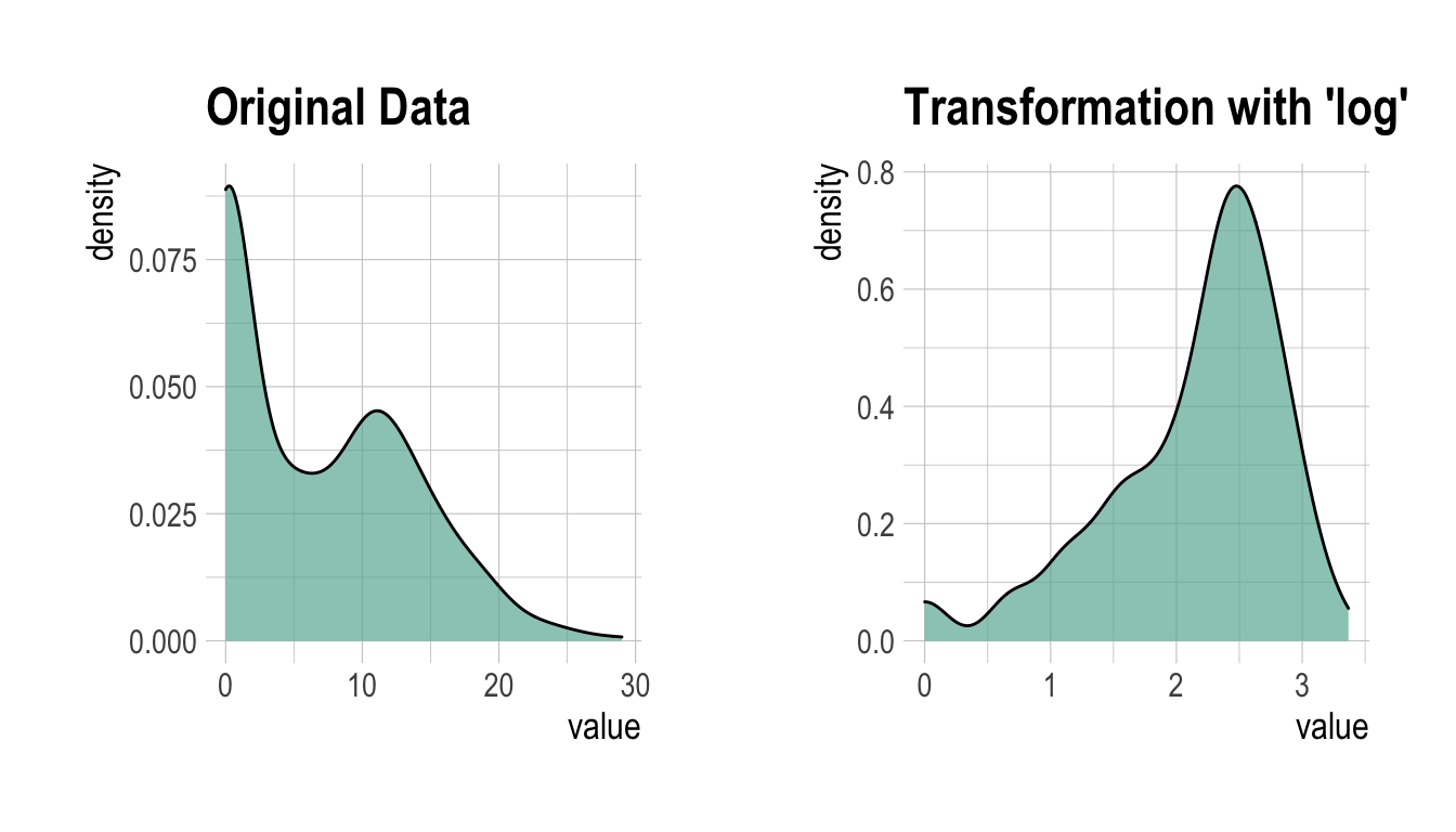
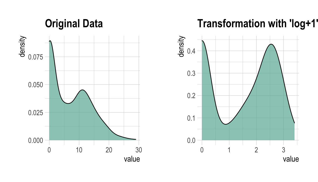
log 변환된 값에 -Inf가 포함되어 있는 것으로 보아 원 데이터에 0이 포함되어 있는 듯하다. 그래서 이번에는 “log+1” 방법으로 변환한다.

Advertising_log = transform(carseats$Advertising, method = "log+1")

# result of transformation
head(Advertising_log)

[1] 2.484907 2.833213 2.397895 1.609438 1.386294 2.639057

# summary of transformation
summary(Advertising_log)

* Resolving Skewness with log+1

* Information of Transformation (before vs after)
            Original Transformation
n        400.0000000   400.00000000
na         0.0000000     0.00000000
mean       6.6350000     1.46247709
sd         6.6503642     1.19436323
se_mean    0.3325182     0.05971816
IQR       12.0000000     2.56494936
skewness   0.6395858    -0.19852549
kurtosis  -0.5451178    -1.66342876
p00        0.0000000     0.00000000
p01        0.0000000     0.00000000
p05        0.0000000     0.00000000
p10        0.0000000     0.00000000
p20        0.0000000     0.00000000
p25        0.0000000     0.00000000
p30        0.0000000     0.00000000
p40        2.0000000     1.09861229
p50        5.0000000     1.79175947
p60        8.4000000     2.23936878
p70       11.0000000     2.48490665
p75       12.0000000     2.56494936
p80       13.0000000     2.63905733
p90       16.0000000     2.83321334
p95       19.0000000     2.99573227
p99       23.0100000     3.17846205
p100      29.0000000     3.40119738

# viz of transformation
plot(Advertising_log)

Binning

binning()을 이용한 개별 변수의 Binning

binning()는 수치형 변수를 비닝하여 범주형 변수로 변환한다. 다음과 같은 type의 비닝을 지원한다.

• “quantile” : 동일한 돗수가 포함되도록 quantile을 이용하여 범주화
• “equal” : 동일한 길이의 구간을 갖도록 범주화
• “pretty” : 적당히 보기 좋은 구간으로 범주화
• “kmeans” : K-means clustering 기법을 이용한 범주화
• “bclust” : Bagged clustering 기법을 이용한 범주화

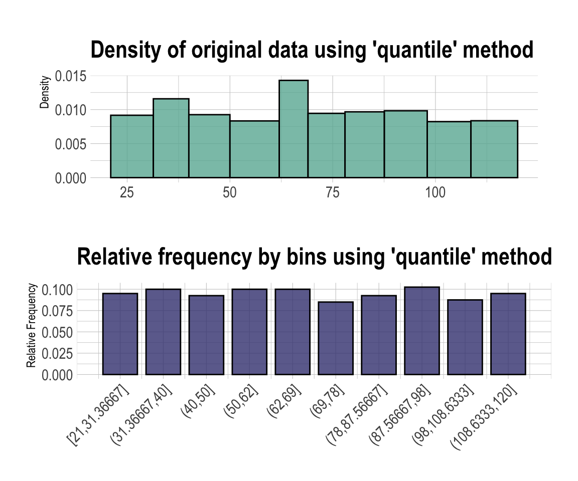
binning()을 이용하여 Income을 비닝하는 몇 가지의 방법을 예시한다.

# Binning the carat variable. default type argument is "quantile"
bin <- binning(carseats$Income)
# Print bins class object
bin

binned type: quantile
number of bins: 10
x
 [21,31.36667]  (31.36667,40]        (40,50]        (50,62] 
            38             40             37             40 
       (62,69]        (69,78]  (78,87.56667]  (87.56667,98] 
            40             34             37             41 
 (98,108.6333] (108.6333,120]           <NA> 
            35             38             20 

# Summarise bins class object
summary(bin)

           levels freq   rate
1   [21,31.36667]   38 0.0950
2   (31.36667,40]   40 0.1000
3         (40,50]   37 0.0925
4         (50,62]   40 0.1000
5         (62,69]   40 0.1000
6         (69,78]   34 0.0850
7   (78,87.56667]   37 0.0925
8   (87.56667,98]   41 0.1025
9   (98,108.6333]   35 0.0875
10 (108.6333,120]   38 0.0950
11           <NA>   20 0.0500

# Plot bins class object
plot(bin)

# Using labels argument
bin <- binning(carseats$Income, nbins = 4,
              labels = c("LQ1", "UQ1", "LQ3", "UQ3"))
bin

binned type: quantile
number of bins: 4
x
 LQ1  UQ1  LQ3  UQ3 <NA> 
  98   97   91   94   20 

# Using another type argument
binning(carseats$Income, nbins = 5, type = "equal")

binned type: equal
number of bins: 5
x
   [21,40.8]  (40.8,60.6]  (60.6,80.4] (80.4,100.2]  (100.2,120] 
          78           68           92           79           63 
        <NA> 
          20 

binning(carseats$Income, nbins = 5, type = "pretty")

binned type: pretty
number of bins: 5
x
  [20,40]   (40,60]   (60,80]  (80,100] (100,120]      <NA> 
       78        68        92        79        63        20 

binning(carseats$Income, nbins = 5, type = "kmeans")

binned type: kmeans
number of bins: 5
x
  [21,38.5] (38.5,56.5] (56.5,75.5] (75.5,97.5]  (97.5,120] 
         72          58          87          86          77 
       <NA> 
         20 

binning(carseats$Income, nbins = 5, type = "bclust")

binned type: bclust
number of bins: 5
x
  [21,37.5] (37.5,55.5] (55.5,78.5] (78.5,95.5]  (95.5,120] 
         69          58         102          69          82 
       <NA> 
         20 

# -------------------------
# Using pipes & dplyr
# -------------------------
library(dplyr)

carseats %>%
 mutate(Income_bin = binning(carseats$Income)) %>%
 group_by(ShelveLoc, Income_bin) %>%
 summarise(freq = n()) %>%
 arrange(desc(freq)) %>%
 head(10)

# A tibble: 10 x 3
# Groups:   ShelveLoc [1]
  ShelveLoc Income_bin     freq
  <fct>     <ord>         <int>
1 Medium    [21,31.36667]    25
2 Medium    (62,69]          23
3 Medium    (50,62]          22
4 Medium    (31.36667,40]    21
# … with 6 more rows

binning_by()을 이용한 Optimal Binning

binning_by()는 수치형 변수를 Optimal Binning하여 범주형 변수로 변환한다. 이 방법은 스코어카드 모형을 개발할때 자주 사용하는 방법이다.

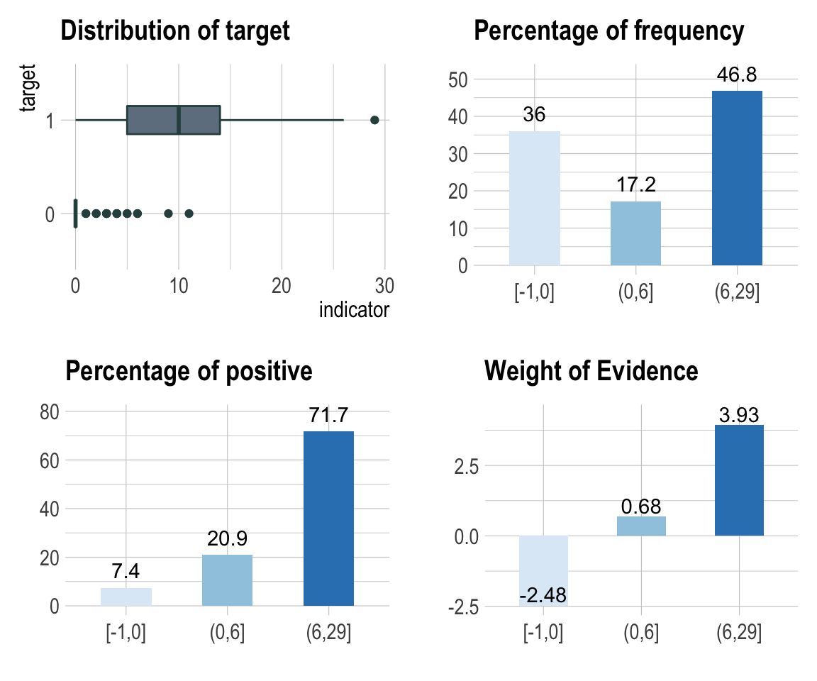
다음의 binning_by() 예제는 US가 binary class를 갖는 target 변수일 경우에 Advertising를 Optimal Binning하는 방법의 예시다.

# optimal binning
bin <- binning_by(carseats, "US", "Advertising")

` US ` ~ ` Advertising `
<environment: 0x7ff8ef6883d8>

bin

binned type: optimal
number of bins: 3
x
[-1,0]  (0,6] (6,29] 
   144     69    187 

# summary optimal_bins class
summary(bin)

── Binning Table ──────────────────────── Several Metrics ── 
     Bin CntRec CntPos CntNeg RatePos RateNeg    Odds      WoE
1 [-1,0]    144     19    125 0.07364 0.88028  0.1520 -2.48101
2  (0,6]     69     54     15 0.20930 0.10563  3.6000  0.68380
3 (6,29]    187    185      2 0.71705 0.01408 92.5000  3.93008
4  Total    400    258    142 1.00000 1.00000  1.8169       NA
       IV     JSD     AUC
1 2.00128 0.20093 0.03241
2 0.07089 0.00869 0.01883
3 2.76272 0.21861 0.00903
4 4.83489 0.42823 0.06028

── General Metrics ───────────────────────────────────────── 
• Gini index                       :  -0.87944
• IV (Jeffrey)                     :  4.83489
• JS (Jensen-Shannon) Divergence   :  0.42823
• Kolmogorov-Smirnov Statistics    :  0.80664
• HHI (Herfindahl-Hirschman Index) :  0.37791
• HHI (normalized)                 :  0.06687
• Cramer's V                       :  0.81863 

── Significance Tests ──────────────────── Chisquare Test ── 
   Bin A  Bin B statistics      p_value
1 [-1,0]  (0,6]   87.67064 7.731349e-21
2  (0,6] (6,29]   34.73349 3.780706e-09

# information value 
attr(bin, "iv")

NULL

# information value table
attr(bin, "ivtable")

NULL

# visualize optimal_bins class
plot(bin, sub = "bins of Advertising variable")

transformation_report()를 이용한 데이터변환 보고서 작성

transformation_report()는 데이터 프레임이나 데이터 프레임을 상속받은 객체(tbl_df, tbl 등)의 모든 변수들에 대해서 데이터변환 보고서를 작성한다.

transformation_report()는 데이터변환 보고서를 다음과 같은 두 개의 형태로 작성한다.

• Latex에 기반한 pdf 파일
• html 파일

보고서의 목차는 다음과 같다.

• 값의 대체
  • 결측치
    • 결측치의 대체 정보
    • (해당 변수들)
  • 이상치
    • 이상치의 대체 정보
    • (해당 변수들)
• 치우침의 해결
  • 치우친 변수들의 정보
    • (해당 변수들)
• 비닝
  • 비닝을 위한 수치형 변수들
  • 비닝
    • (해당 변수들)
  • Optimal 비닝
    • (해당 변수들)

다음은 carseats의 데이터변환 보고서를 작성한다. 파일 형식은 pdf이며, 파일이름은 Transformation_Report.pdf다.

carseats %>%
  transformation_report(target = US)

다음은 transformation.html라는 이름의 html 형식의 보고서를 생성한다.

carseats %>%
  transformation_report(target = US, output_format = "html", 
    output_file = "transformation.html")

데이터변환 보고서는 데이터 변환 과정에 도움을 주기 위한 자동화 보고서다. 보고서 결과를 참고하여 데이터 변환 시나리오를 설계한다.

데이터변환 리포트 내용

pdf 파일의 내용

• 보고서의 표지는 다음 그림과 같다.

Figure 1: 데이터변환 보고서 표지

• 보고서의 차례는 다음 그림과 같다.

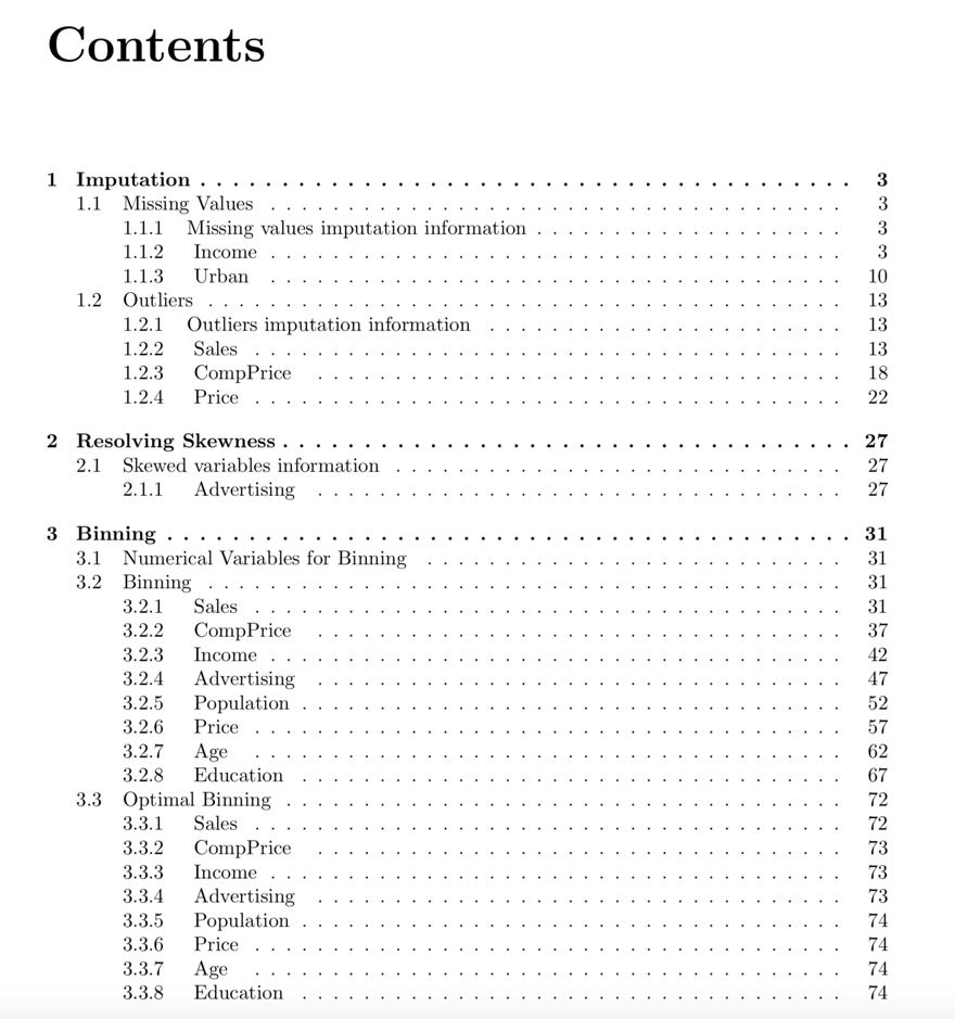
Figure 2: 데이터변환 보고서 차례

• 많은 정보는 보고서에서 표와 시각화 결과로 표현된다. 예시는 다음 그림과 같다.

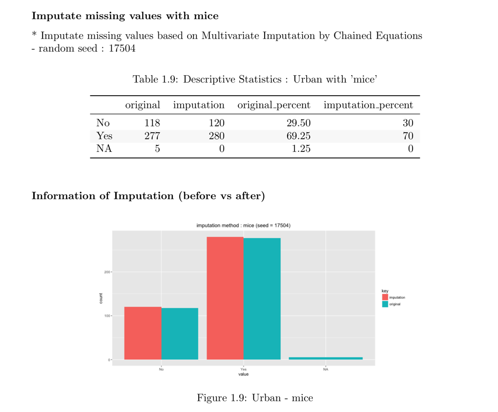
Figure 3: 데이터변환 보고서 도표 및 시각화 예시

html 파일의 내용

• 보고서의 타이틀과 목차는 다음 그림과 같다.

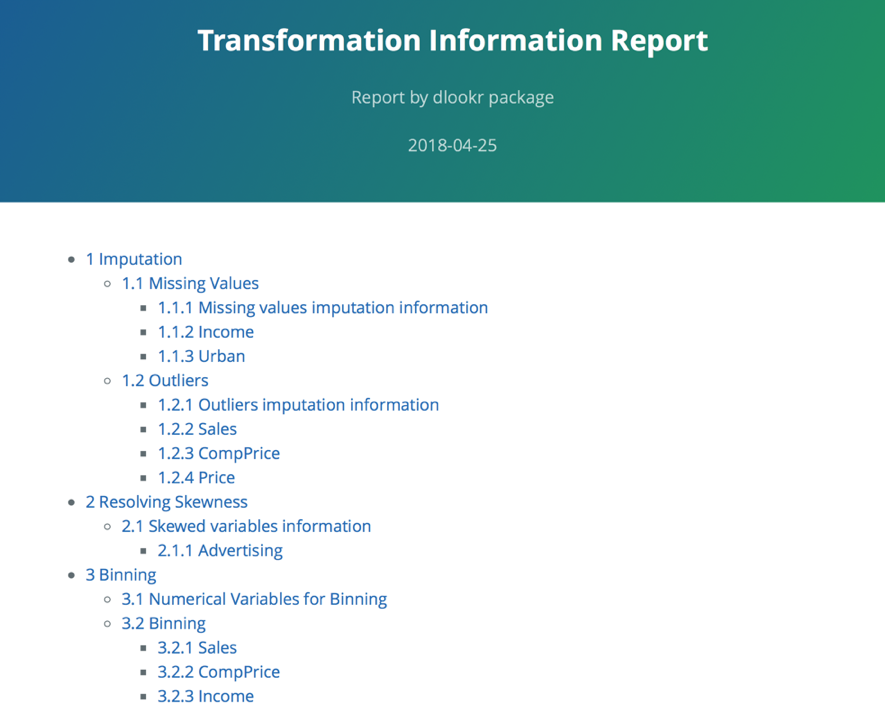
Figure 4: 데이터변환 보고서 타이틀과 목차

• 많은 정보는 보고서에서 표로 표현된다. html 파일에서 표의 예시는 다음 그림과 같다.

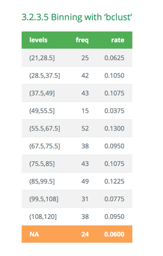
Figure 5: 데이터변환 보고서 도표 예시 (웹)

• 데이터변환 보고서에서 Binning 정보는 시각화 결과를 포함한다. html 파일의 결과는 다음 그림과 같다.

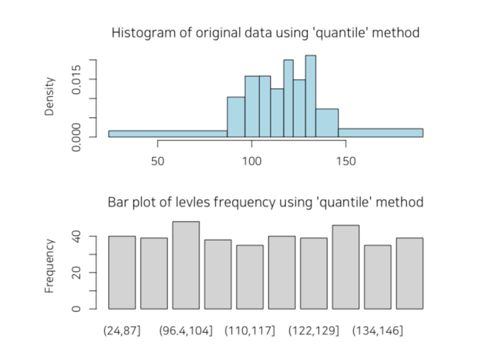
Figure 6: 데이터변환 보고서 Binning 정보 (웹)