Preface
After you have acquired the data, you should do the following:
- Diagnose data quality.
- If there is a problem with data quality,
- The data must be corrected or re-acquired.
- Explore data to understand the data and find scenarios for performing the analysis.
- Derive new variables or perform variable transformations.
The dlookr package makes these steps fast and easy:
- Performs an data diagnosis or automatically generates a data diagnosis report.
- Discover data in a variety of ways, and automatically generate EDA(exploratory data analysis) report.
- Impute missing values and outliers, resolve skewed data, and categorize continuous variables into categorical variables. And generates an automated report to support it.
This document introduces EDA(Exploratory Data Analysis) methods provided by the dlookr package. You will learn how to EDA of tbl_df data that inherits from data.frame and data.frame with functions provided by dlookr.
dlookr increases synergy with dplyr. Particularly in data exploration and data wrangle, it increases the efficiency of the tidyverse package group.
Supported data structures
Data diagnosis supports the following data structures.
- data frame : data.frame class.
- data table : tbl_df class.
- table of DBMS : table of the DBMS through tbl_dbi.
- Use dplyr as the back-end interface for any DBI-compatible database.
datasets
To illustrate the basic use of EDA in the dlookr package, I use a Carseats dataset. Carseats in the ISLR package is a simulated data set containing sales of child car seats at 400 different stores. This data is a data.frame created for the purpose of predicting sales volume.
'data.frame':   400 obs. of  11 variables:
 $ Sales      : num  9.5 11.22 10.06 7.4 4.15 ...
 $ CompPrice  : num  138 111 113 117 141 124 115 136 132 132 ...
 $ Income     : num  73 48 35 100 64 113 105 81 110 113 ...
 $ Advertising: num  11 16 10 4 3 13 0 15 0 0 ...
 $ Population : num  276 260 269 466 340 501 45 425 108 131 ...
 $ Price      : num  120 83 80 97 128 72 108 120 124 124 ...
 $ ShelveLoc  : Factor w/ 3 levels "Bad","Good","Medium": 1 2 3 3 1 1 3 2 3 3 ...
 $ Age        : num  42 65 59 55 38 78 71 67 76 76 ...
 $ Education  : num  17 10 12 14 13 16 15 10 10 17 ...
 $ Urban      : Factor w/ 2 levels "No","Yes": 2 2 2 2 2 1 2 2 1 1 ...
 $ US         : Factor w/ 2 levels "No","Yes": 2 2 2 2 1 2 1 2 1 2 ...
The contents of individual variables are as follows. (Refer to ISLR::Carseats Man page)
- Sales
- Unit sales (in thousands) at each location
- CompPrice
- Price charged by competitor at each location
- Income
- Community income level (in thousands of dollars)
- Advertising
- Local advertising budget for company at each location (in thousands of dollars)
- Population
- Population size in region (in thousands)
- Price
- Price company charges for car seats at each site
- ShelveLoc
- A factor with levels Bad, Good and Medium indicating the quality of the shelving location for the car seats at each site
- Age
- Average age of the local population
- Education
- Education level at each location
- Urban
- A factor with levels No and Yes to indicate whether the store is in an urban or rural location
- US
- A factor with levels No and Yes to indicate whether the store is in the US or not
When data analysis is performed, data containing missing values is frequently encountered. However, ‘Carseats’ is complete data without missing values. So the following script created the missing values and saved them as carseats.
carseats <- ISLR::Carseats

suppressWarnings(RNGversion("3.5.0"))
set.seed(123)
carseats[sample(seq(NROW(carseats)), 20), "Income"] <- NA

suppressWarnings(RNGversion("3.5.0"))
set.seed(456)
carseats[sample(seq(NROW(carseats)), 10), "Urban"] <- NA
Exploratory Data Analysis
dlookr can help to understand the distribution of data by calculating descriptive statistics of numerical data. In addition, correlation between variables is identified and normality test is performed. It also identifies the relationship between target variables and independent variables.:
The following is a list of the EDA functions included in the dlookr package.:
describe()provides descriptive statistics for numerical data.normality()andplot_normality()perform normalization and visualization of numerical data.correlate()andplot_correlate()calculate the correlation coefficient between two numerical data and provide visualization.target_by()defines the target variable andrelate()describes the relationship with the variables of interest corresponding to the target variable.plot.relate()visualizes the relationship to the variable of interest corresponding to the destination variable.eda_report()performs an exploratory data analysis and reports the results.
Univariate data EDA
Calculating descriptive statistics using describe()
describe() computes descriptive statistics for numerical data. The descriptive statistics help determine the distribution of numerical variables. Like function of dplyr, the first argument is the tibble (or data frame). The second and subsequent arguments refer to variables within that data frame.
The variables of the tbl_df object returned by describe() are as follows.
n: number of observations excluding missing valuesna: number of missing valuesmean: arithmetic averagesd: standard deviationse_mean: standard error mean. sd/sqrt(n)IQR: interquartile range (Q3-Q1)skewness: skewnesskurtosis: kurtosisp25: Q1. 25% percentilep50: median. 50% percentilep75: Q3. 75% percentilep01,p05,p10,p20,p30: 1%, 5%, 20%, 30% percentilesp40,p60,p70,p80: 40%, 60%, 70%, 80% percentilesp90,p95,p99,p100: 90%, 95%, 99%, 100% percentiles
For example, describe() can computes the statistics of all numerical variables in carseats:
describe(carseats)
# A tibble: 8 x 26
  variable        n    na   mean    sd se_mean   IQR skewness kurtosis
  <chr>       <int> <int>  <dbl> <dbl>   <dbl> <dbl>    <dbl>    <dbl>
1 Sales         400     0   7.50  2.82   0.141  3.93   0.186   -0.0809
2 CompPrice     400     0 125.   15.3    0.767 20     -0.0428   0.0417
3 Income        380    20  68.9  28.1    1.44  48.2    0.0449  -1.09
4 Advertising   400     0   6.64  6.65   0.333 12      0.640   -0.545
# … with 4 more rows, and 17 more variables: p00 <dbl>, p01 <dbl>,
#   p05 <dbl>, p10 <dbl>, p20 <dbl>, p25 <dbl>, p30 <dbl>, p40 <dbl>,
#   p50 <dbl>, p60 <dbl>, p70 <dbl>, p75 <dbl>, p80 <dbl>, p90 <dbl>,
# p95 <dbl>, p99 <dbl>, p100 <dbl>skewness: The left-skewed distribution data that is the variables with large positive skewness should consider the log or sqrt transformations to follow the normal distribution. The variablesAdvertisingseem to need to consider variable transformation.meanandsd,se_mean: ThePopulationwith a largestandard error of the mean(se_mean) has low representativeness of thearithmetic mean(mean). Thestandard deviation(sd) is much larger than the arithmetic average.
The following explains the descriptive statistics only for a few selected variables.:
# Select columns by name
describe(carseats, Sales, CompPrice, Income)
# A tibble: 3 x 26
  variable      n    na   mean    sd se_mean   IQR skewness kurtosis
  <chr>     <int> <int>  <dbl> <dbl>   <dbl> <dbl>    <dbl>    <dbl>
1 Sales       400     0   7.50  2.82   0.141  3.93   0.186   -0.0809
2 CompPrice   400     0 125.   15.3    0.767 20     -0.0428   0.0417
3 Income      380    20  68.9  28.1    1.44  48.2    0.0449  -1.09
# … with 17 more variables: p00 <dbl>, p01 <dbl>, p05 <dbl>,
#   p10 <dbl>, p20 <dbl>, p25 <dbl>, p30 <dbl>, p40 <dbl>, p50 <dbl>,
#   p60 <dbl>, p70 <dbl>, p75 <dbl>, p80 <dbl>, p90 <dbl>, p95 <dbl>,
#   p99 <dbl>, p100 <dbl>
# Select all columns between year and day (include)
describe(carseats, Sales:Income)
# A tibble: 3 x 26
  variable      n    na   mean    sd se_mean   IQR skewness kurtosis
  <chr>     <int> <int>  <dbl> <dbl>   <dbl> <dbl>    <dbl>    <dbl>
1 Sales       400     0   7.50  2.82   0.141  3.93   0.186   -0.0809
2 CompPrice   400     0 125.   15.3    0.767 20     -0.0428   0.0417
3 Income      380    20  68.9  28.1    1.44  48.2    0.0449  -1.09
# … with 17 more variables: p00 <dbl>, p01 <dbl>, p05 <dbl>,
#   p10 <dbl>, p20 <dbl>, p25 <dbl>, p30 <dbl>, p40 <dbl>, p50 <dbl>,
#   p60 <dbl>, p70 <dbl>, p75 <dbl>, p80 <dbl>, p90 <dbl>, p95 <dbl>,
#   p99 <dbl>, p100 <dbl>
# Select all columns except those from year to day (exclude)
describe(carseats, -(Sales:Income))
# A tibble: 5 x 26
  variable       n    na   mean     sd se_mean   IQR skewness kurtosis
  <chr>      <int> <int>  <dbl>  <dbl>   <dbl> <dbl>    <dbl>    <dbl>
1 Advertisi…   400     0   6.64   6.65   0.333  12     0.640    -0.545
2 Population   400     0 265.   147.     7.37  260.   -0.0512   -1.20
3 Price        400     0 116.    23.7    1.18   31    -0.125     0.452
4 Age          400     0  53.3   16.2    0.810  26.2  -0.0772   -1.13
# … with 1 more row, and 17 more variables: p00 <dbl>, p01 <dbl>,
#   p05 <dbl>, p10 <dbl>, p20 <dbl>, p25 <dbl>, p30 <dbl>, p40 <dbl>,
#   p50 <dbl>, p60 <dbl>, p70 <dbl>, p75 <dbl>, p80 <dbl>, p90 <dbl>,
#   p95 <dbl>, p99 <dbl>, p100 <dbl>
The describe() function can be sorted by left or right skewed size(skewness) using dplyr.:
carseats %>%
  describe() %>%
  select(variable, skewness, mean, p25, p50, p75) %>%
  filter(!is.na(skewness)) %>%
  arrange(desc(abs(skewness)))
# A tibble: 8 x 6
  variable    skewness   mean    p25    p50    p75
  <chr>          <dbl>  <dbl>  <dbl>  <dbl>  <dbl>
1 Advertising   0.640    6.64   0      5     12
2 Sales         0.186    7.50   5.39   7.49   9.32
3 Price        -0.125  116.   100    117    131
4 Age          -0.0772  53.3   39.8   54.5   66
# … with 4 more rows
The describe() function supports the group_by() function syntax of the dplyr package.
carseats %>%
  group_by(US) %>%
  describe(Sales, Income)
# A tibble: 4 x 27
  variable US        n    na  mean    sd se_mean   IQR skewness
  <chr>    <fct> <int> <int> <dbl> <dbl>   <dbl> <dbl>    <dbl>
1 Income   No      130    12 65.8  28.2    2.48  50      0.100
2 Income   Yes     250     8 70.4  27.9    1.77  48      0.0199
3 Sales    No      142     0  6.82  2.60   0.218  3.44   0.323
4 Sales    Yes     258     0  7.87  2.88   0.179  4.23   0.0760
# … with 18 more variables: kurtosis <dbl>, p00 <dbl>, p01 <dbl>,
#   p05 <dbl>, p10 <dbl>, p20 <dbl>, p25 <dbl>, p30 <dbl>, p40 <dbl>,
#   p50 <dbl>, p60 <dbl>, p70 <dbl>, p75 <dbl>, p80 <dbl>, p90 <dbl>,
#   p95 <dbl>, p99 <dbl>, p100 <dbl>
carseats %>%
group_by(US, Urban) %>%
describe(Sales, Income)
# A tibble: 12 x 28
  variable US    Urban     n    na  mean    sd se_mean   IQR skewness
  <chr>    <fct> <fct> <int> <int> <dbl> <dbl>   <dbl> <dbl>    <dbl>
1 Income   No    No       42     4  60.2  29.1    4.49  45.2   0.408
2 Income   No    Yes      84     8  69.5  27.4    2.99  47    -0.0497
3 Income   No    <NA>      4     0  48.2  24.7   12.3   40.8  -0.0496
4 Income   Yes   No       65     4  70.5  29.9    3.70  48     0.0736
# … with 8 more rows, and 18 more variables: kurtosis <dbl>,
#   p00 <dbl>, p01 <dbl>, p05 <dbl>, p10 <dbl>, p20 <dbl>, p25 <dbl>,
#   p30 <dbl>, p40 <dbl>, p50 <dbl>, p60 <dbl>, p70 <dbl>, p75 <dbl>,
#   p80 <dbl>, p90 <dbl>, p95 <dbl>, p99 <dbl>, p100 <dbl>
Test of normality on numeric variables using normality()
normality() performs a normality test on numerical data. Shapiro-Wilk normality test is performed. When the number of observations is greater than 5000, it is tested after extracting 5000 samples by random simple sampling.
The variables of tbl_df object returned by normality() are as follows.
statistic: Statistics of the Shapiro-Wilk testp_value: p-value of the Shapiro-Wilk testsample: Number of sample observations performed Shapiro-Wilk test
normality() performs the normality test for all numerical variables of carseats as follows.:
normality(carseats)
# A tibble: 8 x 4
  vars        statistic  p_value sample
  <chr>           <dbl>    <dbl>  <dbl>
1 Sales           0.995 2.54e- 1    400
2 CompPrice       0.998 9.77e- 1    400
3 Income          0.961 1.52e- 8    400
4 Advertising     0.874 1.49e-17    400
# … with 4 more rows
The following example performs a normality test on only a few selected variables.
# Select columns by name
normality(carseats, Sales, CompPrice, Income)
# A tibble: 3 x 4
  vars      statistic      p_value sample
  <chr>         <dbl>        <dbl>  <dbl>
1 Sales         0.995 0.254           400
2 CompPrice     0.998 0.977           400
3 Income        0.961 0.0000000152    400
# Select all columns between year and day (inclusive)
normality(carseats, Sales:Income)
# A tibble: 3 x 4
  vars      statistic      p_value sample
  <chr>         <dbl>        <dbl>  <dbl>
1 Sales         0.995 0.254           400
2 CompPrice     0.998 0.977           400
3 Income        0.961 0.0000000152    400
# Select all columns except those from year to day (inclusive)
normality(carseats, -(Sales:Income))
# A tibble: 5 x 4
  vars        statistic  p_value sample
  <chr>           <dbl>    <dbl>  <dbl>
1 Advertising     0.874 1.49e-17    400
2 Population      0.952 4.08e-10    400
3 Price           0.996 3.90e- 1    400
4 Age             0.957 1.86e- 9    400
# … with 1 more row
You can use dplyr to sort variables that do not follow a normal distribution in order of p_value:
# A tibble: 5 x 4
  vars        statistic  p_value sample
  <chr>           <dbl>    <dbl>  <dbl>
1 Advertising     0.874 1.49e-17    400
2 Education       0.924 2.43e-13    400
3 Population      0.952 4.08e-10    400
4 Age             0.957 1.86e- 9    400
# … with 1 more row
In particular, the Advertising variable is considered to be the most out of the normal distribution.
The normality() function supports the group_by() function syntax in the dplyr package.
# A tibble: 6 x 6
  variable ShelveLoc US    statistic p_value sample
  <chr>    <fct>     <fct>     <dbl>   <dbl>  <dbl>
1 Income   Bad       No        0.969  0.470      34
2 Income   Bad       Yes       0.958  0.0343     62
3 Income   Good      No        0.902  0.0328     24
4 Income   Good      Yes       0.955  0.0296     61
# … with 2 more rows
The Income variable does not follow the normal distribution. However, the case where US is No and ShelveLoc is Good and Bad at the significance level of 0.01, it follows the normal distribution.
The following example performs normality test of log(Income) for each combination of ShelveLoc and US categorical variables to search for variables that follow the normal distribution.
carseats %>%
  mutate(log_income = log(Income)) %>%
  group_by(ShelveLoc, US) %>%
  normality(log_income) %>%
  filter(p_value > 0.01)
# A tibble: 1 x 6
  variable   ShelveLoc US    statistic p_value sample
  <chr>      <fct>     <fct>     <dbl>   <dbl>  <dbl>
1 log_income Bad       No        0.940  0.0737     34
Visualization of normality of numerical variables using plot_normality()
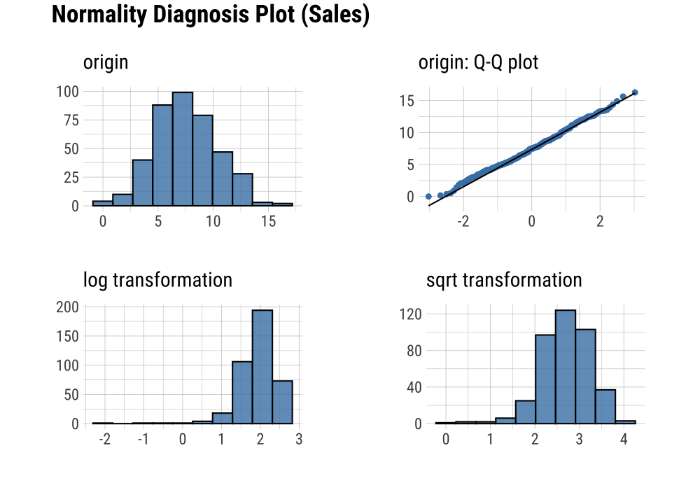
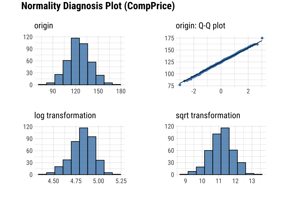
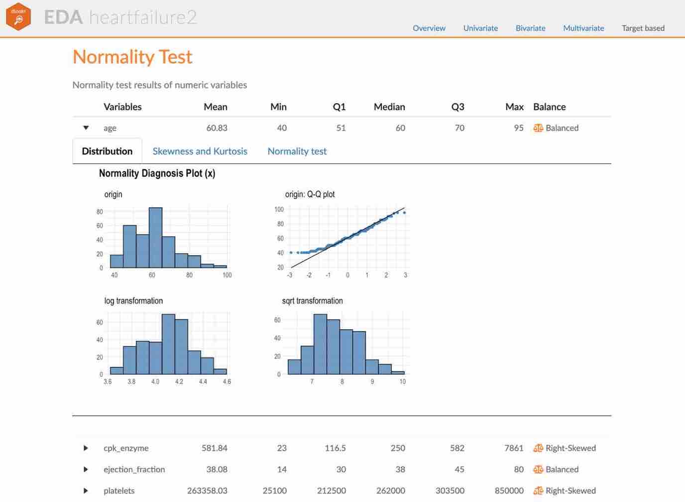
plot_normality() visualizes the normality of numeric data.
The information visualized by plot_normality() is as follows.:
Histogram of original dataQ-Q plot of original datahistogram of log transformed dataHistogram of square root transformed data
In the data analysis process, it often encounters numerical data that follows the power-law distribution. Since the numerical data that follows the power-law distribution is converted into a normal distribution by performing the log or sqrt transformation, so draw a histogram of the log and sqrt transformed data.
plot_normality() can also specify several variables like normality() function.
# Select columns by name
plot_normality(carseats, Sales, CompPrice)
The plot_normality() function also supports the group_by() function syntax in the dplyr package.
EDA of bivariate data
Calculation of correlation coefficient using correlate()
correlate() calculates the correlation coefficient of all combinations of carseats numerical variables as follows:
correlate(carseats)
# A tibble: 56 x 3
  var1        var2  coef_corr
  <fct>       <fct>     <dbl>
1 CompPrice   Sales    0.0641
2 Income      Sales    0.151
3 Advertising Sales    0.270
4 Population  Sales    0.0505
# … with 52 more rows
The following example performs a normality test only on combinations that include several selected variables.
# Select columns by name
correlate(carseats, Sales, CompPrice, Income)
# A tibble: 21 x 3
  var1      var2      coef_corr
  <fct>     <fct>         <dbl>
1 CompPrice Sales        0.0641
2 Income    Sales        0.151
3 Sales     CompPrice    0.0641
4 Income    CompPrice   -0.0761
# … with 17 more rows
# Select all columns between year and day (include)
correlate(carseats, Sales:Income)
# A tibble: 21 x 3
  var1      var2      coef_corr
  <fct>     <fct>         <dbl>
1 CompPrice Sales        0.0641
2 Income    Sales        0.151
3 Sales     CompPrice    0.0641
4 Income    CompPrice   -0.0761
# … with 17 more rows
# Select all columns except those from year to day (exclude)
correlate(carseats, -(Sales:Income))
# A tibble: 35 x 3
  var1        var2  coef_corr
  <fct>       <fct>     <dbl>
1 Advertising Sales    0.270
2 Population  Sales    0.0505
3 Price       Sales   -0.445
4 Age         Sales   -0.232
# … with 31 more rows
correlate() produces two pairs of variables. So the following example uses filter() to get the correlation coefficient for a pair of variable combinations:
carseats %>%
  correlate(Sales:Income) %>%
  filter(as.integer(var1) > as.integer(var2))
# A tibble: 3 x 3
  var1      var2      coef_corr
  <fct>     <fct>         <dbl>
1 CompPrice Sales        0.0641
2 Income    Sales        0.151
3 Income    CompPrice   -0.0761
The correlate() also supports the group_by() function syntax in the dplyr package.
carseats %>%
  filter(ShelveLoc == "Good") %>%
  group_by(Urban, US) %>%
  correlate(Sales) %>%
  filter(abs(coef_corr) > 0.5)
# A tibble: 10 x 5
  Urban US    var1  var2       coef_corr
  <fct> <fct> <fct> <fct>          <dbl>
1 No    No    Sales Population    -0.530
2 No    No    Sales Price         -0.838
3 No    Yes   Sales Price         -0.630
4 Yes   No    Sales Price         -0.833
# … with 6 more rows
Visualization of the correlation matrix using plot_correlate()
plot_correlate() visualizes the correlation matrix.
plot_correlate(carseats)
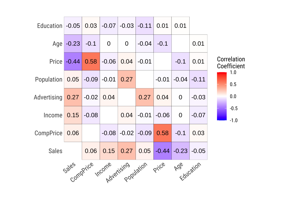
plot_correlate() can also specify multiple variables, like the correlate() function. The following is a visualization of the correlation matrix including several selected variables.
# Select columns by name
plot_correlate(carseats, Sales, Price)
The plot_correlate() function also supports the group_by() function syntax in the dplyr package.
EDA based on target variable
Definition of target variable
To perform EDA based on target variable, you need to create a target_by class object. target_by() creates a target_by class with an object inheriting data.frame or data.frame. target_by() is similar to group_by() in dplyr which creates grouped_df. The difference is that you specify only one variable.
The following is an example of specifying US as target variable in carseats data.frame.:
categ <- target_by(carseats, US)
EDA when target variable is categorical variable
Let’s perform EDA when the target variable is a categorical variable. When the categorical variable US is the target variable, we examine the relationship between the target variable and the predictor.
Cases where predictors are numeric variable
relate() shows the relationship between the target variable and the predictor. The following example shows the relationship between Sales and the target variable US. The predictor Sales is a numeric variable. In this case, the descriptive statistics are shown for each level of the target variable.
# If the variable of interest is a numerical variable
cat_num <- relate(categ, Sales)
cat_num
# A tibble: 3 x 27
  variable US        n    na  mean    sd se_mean   IQR skewness
  <chr>    <fct> <int> <int> <dbl> <dbl>   <dbl> <dbl>    <dbl>
1 Sales    No      142     0  6.82  2.60   0.218  3.44   0.323
2 Sales    Yes     258     0  7.87  2.88   0.179  4.23   0.0760
3 Sales    total   400     0  7.50  2.82   0.141  3.93   0.186
# … with 18 more variables: kurtosis <dbl>, p00 <dbl>, p01 <dbl>,
#   p05 <dbl>, p10 <dbl>, p20 <dbl>, p25 <dbl>, p30 <dbl>, p40 <dbl>,
#   p50 <dbl>, p60 <dbl>, p70 <dbl>, p75 <dbl>, p80 <dbl>, p90 <dbl>,
# p95 <dbl>, p99 <dbl>, p100 <dbl>summary(cat_num)
variable US n na
Length:3 No :1 Min. :142.0 Min. :0
Class :character Yes :1 1st Qu.:200.0 1st Qu.:0
Mode :character total:1 Median :258.0 Median :0
Mean :266.7 Mean :0
3rd Qu.:329.0 3rd Qu.:0
Max. :400.0 Max. :0
mean sd se_mean IQR
Min. :6.823 Min. :2.603 Min. :0.1412 Min. :3.442
1st Qu.:7.160 1st Qu.:2.713 1st Qu.:0.1602 1st Qu.:3.686
Median :7.496 Median :2.824 Median :0.1791 Median :3.930
Mean :7.395 Mean :2.768 Mean :0.1796 Mean :3.866
3rd Qu.:7.682 3rd Qu.:2.851 3rd Qu.:0.1988 3rd Qu.:4.077
Max. :7.867 Max. :2.877 Max. :0.2184 Max. :4.225
skewness kurtosis p00
Min. :0.07603 Min. :-0.32638 Min. :0.0000
1st Qu.:0.13080 1st Qu.:-0.20363 1st Qu.:0.0000
Median :0.18556 Median :-0.08088 Median :0.0000
Mean :0.19489 Mean : 0.13350 Mean :0.1233
3rd Qu.:0.25432 3rd Qu.: 0.36344 3rd Qu.:0.1850
Max. :0.32308 Max. : 0.80776 Max. :0.3700
p01 p05 p10 p20
Min. :0.4675 Min. :3.147 Min. :3.917 Min. :4.754
1st Qu.:0.6868 1st Qu.:3.148 1st Qu.:4.018 1st Qu.:4.910
Median :0.9062 Median :3.149 Median :4.119 Median :5.066
Mean :1.0072 Mean :3.183 Mean :4.073 Mean :5.051
3rd Qu.:1.2771 3rd Qu.:3.200 3rd Qu.:4.152 3rd Qu.:5.199
Max. :1.6480 Max. :3.252 Max. :4.184 Max. :5.332
p25 p30 p40 p50
Min. :5.080 Min. :5.306 Min. :5.994 Min. :6.660
1st Qu.:5.235 1st Qu.:5.587 1st Qu.:6.301 1st Qu.:7.075
Median :5.390 Median :5.867 Median :6.608 Median :7.490
Mean :5.411 Mean :5.775 Mean :6.506 Mean :7.313
3rd Qu.:5.576 3rd Qu.:6.010 3rd Qu.:6.762 3rd Qu.:7.640
Max. :5.763 Max. :6.153 Max. :6.916 Max. :7.790
p60 p70 p75 p80
Min. :7.496 Min. :7.957 Min. :8.523 Min. : 8.772
1st Qu.:7.787 1st Qu.:8.386 1st Qu.:8.921 1st Qu.: 9.265
Median :8.078 Median :8.815 Median :9.320 Median : 9.758
Mean :8.076 Mean :8.740 Mean :9.277 Mean : 9.665
3rd Qu.:8.366 3rd Qu.:9.132 3rd Qu.:9.654 3rd Qu.:10.111
Max. :8.654 Max. :9.449 Max. :9.988 Max. :10.464
p90 p95 p99 p100
Min. : 9.349 Min. :11.28 Min. :13.64 Min. :14.90
1st Qu.:10.325 1st Qu.:11.86 1st Qu.:13.78 1st Qu.:15.59
Median :11.300 Median :12.44 Median :13.91 Median :16.27
Mean :10.795 Mean :12.08 Mean :13.86 Mean :15.81
3rd Qu.:11.518 3rd Qu.:12.49 3rd Qu.:13.97 3rd Qu.:16.27
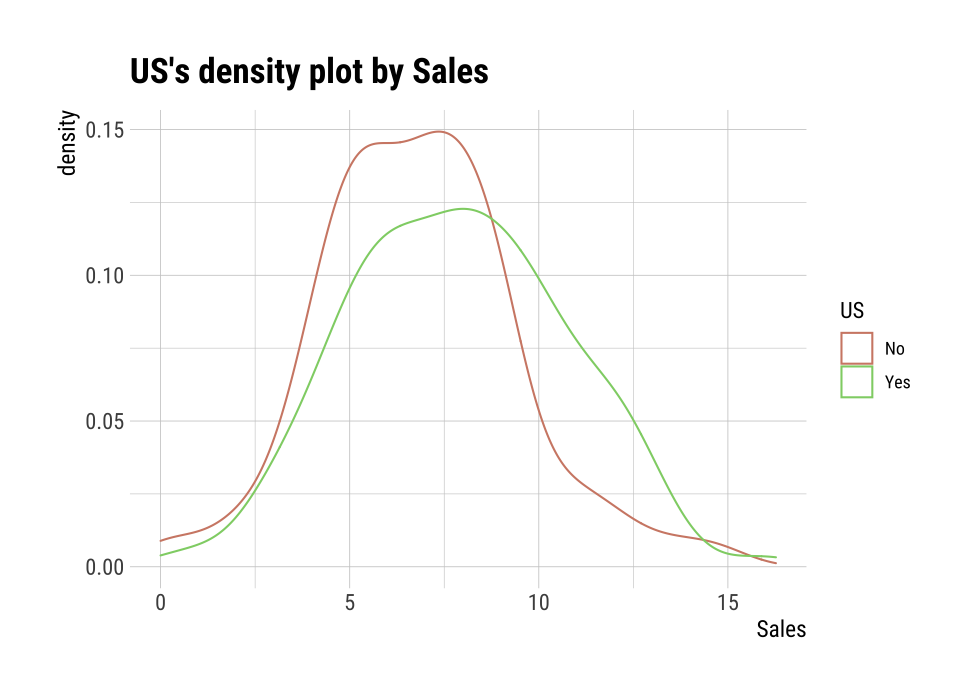
Max. :11.736 Max. :12.54 Max. :14.03 Max. :16.27 plot() visualizes the relate class object created by relate() as the relationship between the target variable and the predictor variable. The relationship between US and Sales is visualized by density plot.
plot(cat_num)
Cases where predictors are categorical variable
The following example shows the relationship between ShelveLoc and the target variable US. The predictor variable ShelveLoc is a categorical variable. In this case, it shows the contingency table of two variables. The summary() function performs independence test on the contingency table.
# If the variable of interest is a categorical variable
cat_cat <- relate(categ, ShelveLoc)
cat_cat
     ShelveLoc
US    Bad Good Medium
  No   34   24     84
Yes 62 61 135summary(cat_cat)
Call: xtabs(formula = formula_str, data = data, addNA = TRUE)
Number of cases in table: 400
Number of factors: 2
Test for independence of all factors:
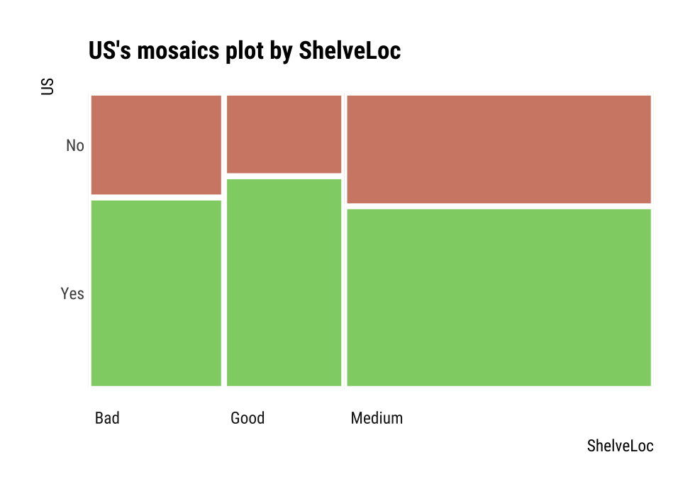
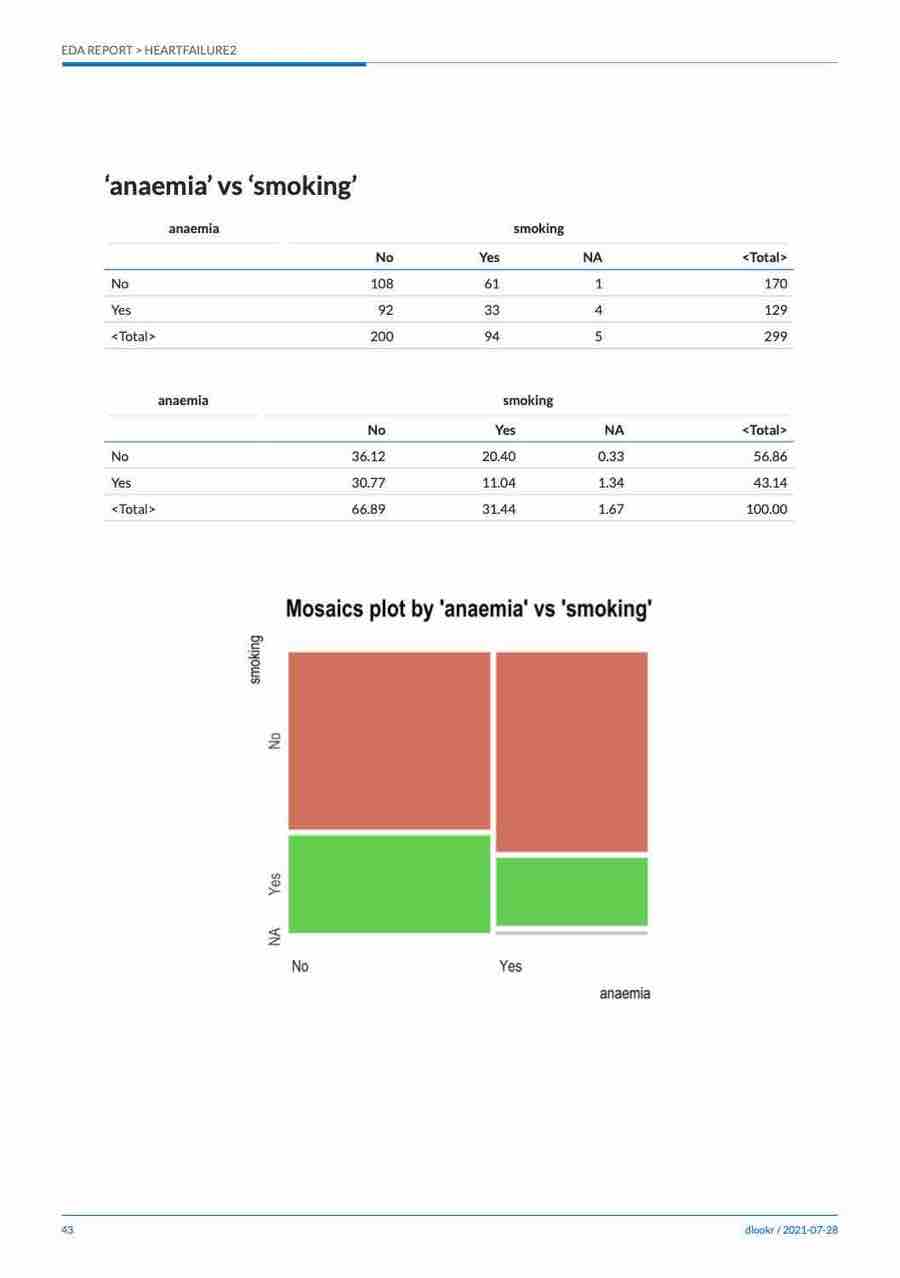
Chisq = 2.7397, df = 2, p-value = 0.2541plot() visualizes the relationship between the target variable and the predictor. The relationship between US and ShelveLoc is represented by a mosaics plot.
plot(cat_cat)
EDA when target variable is numerical variable
Let’s perform EDA when the target variable is numeric. When the numeric variable Sales is the target variable, we examine the relationship between the target variable and the predictor.
# If the variable of interest is a numerical variable
num <- target_by(carseats, Sales)
Cases where predictors are numeric variable
The following example shows the relationship between Price and the target variable Sales. The predictor variable Price is a numeric variable. In this case, it shows the result of a simple linear model of the target ~ predictor formula. The summary() function expresses the details of the model.
# If the variable of interest is a numerical variable
num_num <- relate(num, Price)
num_num
Call:
lm(formula = formula_str, data = data)

Coefficients:
(Intercept)        Price
13.64192 -0.05307 summary(num_num)
Call:
lm(formula = formula_str, data = data)
Residuals:
Min 1Q Median 3Q Max
-6.5224 -1.8442 -0.1459 1.6503 7.5108
Coefficients:
Estimate Std. Error t value Pr(>|t|)
(Intercept) 13.641915 0.632812 21.558 <2e-16 ***
Price -0.053073 0.005354 -9.912 <2e-16 ***
---
Signif. codes: 0 '***' 0.001 '**' 0.01 '*' 0.05 '.' 0.1 ' ' 1
Residual standard error: 2.532 on 398 degrees of freedom
Multiple R-squared: 0.198, Adjusted R-squared: 0.196
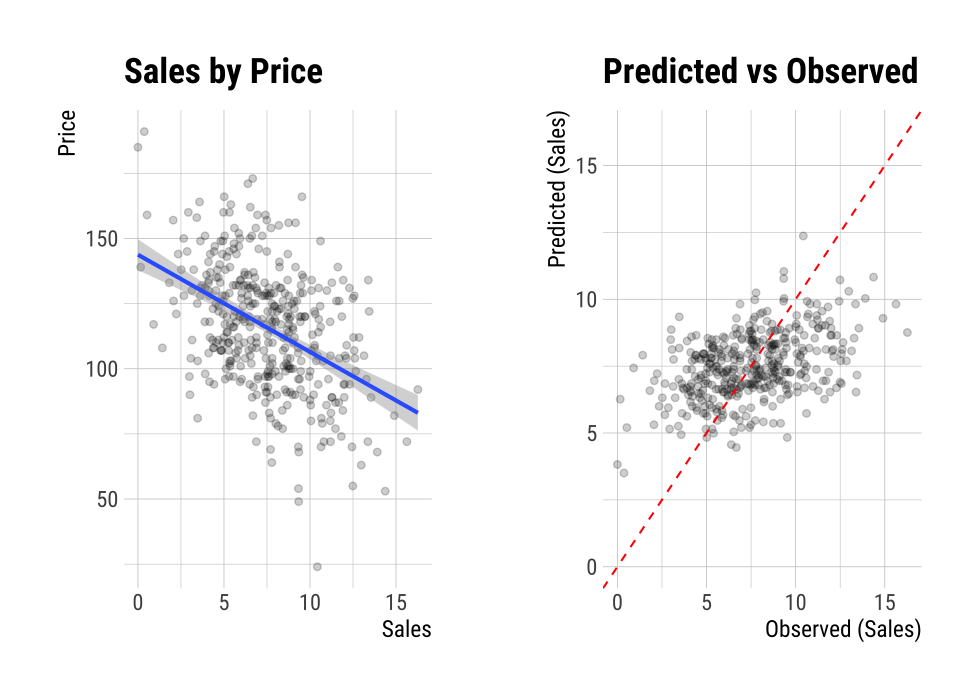
F-statistic: 98.25 on 1 and 398 DF, p-value: < 2.2e-16plot() visualizes the relationship between the target and predictor variables. The relationship between Sales and Price is visualized with a scatter plot. The figure on the left shows the scatter plot of Sales and Price and the confidence interval of the regression line and regression line. The figure on the right shows the relationship between the original data and the predicted values of the linear model as a scatter plot. If there is a linear relationship between the two variables, the scatter plot of the observations converges on the red diagonal line.
plot(num_num)
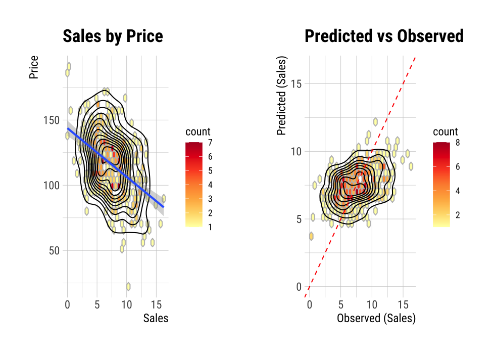
The scatter plot of the data with a large number of observations is output as overlapping points. This makes it difficult to judge the relationship between the two variables. It also takes a long time to perform the visualization. In this case, the above problem can be solved by hexabin plot.
In plot(), the hex_thres argument provides a basis for drawing hexabin plot. If the number of observations is greater than hex_thres, draw a hexabin plot.
The following example visualizes the hexabin plot rather than the scatter plot by specifying 350 for the hex_thres argument. This is because the number of observations is 400.
plot(num_num, hex_thres = 350)
Cases where predictors are categorical variable
The following example shows the relationship between ShelveLoc and the target variable Sales. The predictor ShelveLoc is a categorical variable and shows the result of one-way ANOVA of target ~ predictor relationship. The results are expressed in terms of ANOVA. The summary() function shows the regression coefficients for each level of the predictor. In other words, it shows detailed information about simple regression analysis of target ~ predictor relationship.
# If the variable of interest is a categorical variable
num_cat <- relate(num, ShelveLoc)
num_cat
Analysis of Variance Table

Response: Sales
           Df Sum Sq Mean Sq F value    Pr(>F)
ShelveLoc   2 1009.5  504.77   92.23 < 2.2e-16 ***
Residuals 397 2172.7    5.47
---
Signif. codes: 0 '***' 0.001 '**' 0.01 '*' 0.05 '.' 0.1 ' ' 1summary(num_cat)
Call:
lm(formula = formula(formula_str), data = data)
Residuals:
Min 1Q Median 3Q Max
-7.3066 -1.6282 -0.0416 1.5666 6.1471
Coefficients:
Estimate Std. Error t value Pr(>|t|)
(Intercept) 5.5229 0.2388 23.131 < 2e-16 ***
ShelveLocGood 4.6911 0.3484 13.464 < 2e-16 ***
ShelveLocMedium 1.7837 0.2864 6.229 1.2e-09 ***
---
Signif. codes: 0 '***' 0.001 '**' 0.01 '*' 0.05 '.' 0.1 ' ' 1
Residual standard error: 2.339 on 397 degrees of freedom
Multiple R-squared: 0.3172, Adjusted R-squared: 0.3138
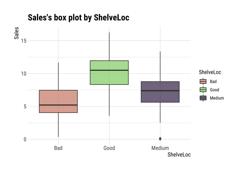
F-statistic: 92.23 on 2 and 397 DF, p-value: < 2.2e-16plot() visualizes the relationship between the target variable and the predictor. The relationship between Sales and ShelveLoc is represented by a box plot.
plot(num_cat)
Automated report
dlookr provides two automated EDA reports:
- Web page-based dynamic reports can perform in-depth analysis through visualization and statistical tables.
- Static reports generated as pdf files or html files can be archived as output of data analysis.
Create a dynamic report using eda_web_report()
eda_web_report() create dynamic report for object inherited from data.frame(tbl_df, tbl, etc) or data.frame.
Contents of dynamic web report
The contents of the report are as follows.:
- Overview
- Data Structures
- Data Types
- Job Informations
- Univariate Analysis
- Descriptive Statistics
- Normality Test
- Bivariate Analysis
- Compare Numerical Variables
- Compare Categorical Variables
- Multivariate Analysis
- Correlation Analysis
- Correlation Matrix
- Correlation Plot
- Correlation Analysis
- Target based Analysis
- Grouped Numerical Variables
- Grouped Categorical Variables
- Grouped Correlation
Some arguments for dynamic web report
eda_web_report() generates various reports with the following arguments.
- target
- target variable
- output_file
- name of generated file.
- output_dir
- name of directory to generate report file.
- title
- title of report.
- subtitle
- subtitle of report.
- author
- author of report.
- title_color
- color of title.
- logo_img
- name of logo image file on top left.
- create_date
- The date on which the report is generated.
- theme
- name of theme for report. support “orange” and “blue”.
- sample_percent
- Sample percent of data for performing EDA.
The following script creates a EDA report for the data.frame class object, heartfailure.
heartfailure %>%
  eda_web_report(target = "death_event", subtitle = "heartfailure",
                 output_dir = "./", output_file = "EDA.html", theme = "blue")
Screenshot of dynamic report
- The dynamic contents of the report is shown in the following figure.:
(#fig:eda_web_title)The part of the report
Create a EDA report using eda_paged_report()
eda_paged_report() create static report for object inherited from data.frame(tbl_df, tbl, etc) or data.frame.
Contents of static paged report
The contents of the report are as follows.:
- Overview
- Data Structures
- Job Informations
- Univariate Analysis
- Descriptive Statistics
- Numerical Variables
- Categorical Variables
- Normality Test
- Descriptive Statistics
- Bivariate Analysis
- Compare Numerical Variables
- Compare Categorical Variables
- Multivariate Analysis
- Correlation Analysis
- Correlation Coefficient Matrix
- Correlation Plot
- Correlation Analysis
- Target based Analysis
- Grouped Numerical Variables
- Grouped Categorical Variables
- Grouped Correlation
Some arguments for static paged report
eda_paged_report() generates various reports with the following arguments.
- target
- target variable
- output_format
- report output type. Choose either “pdf” and “html”.
- output_file
- name of generated file.
- output_dir
- name of directory to generate report file.
- title
- title of report.
- subtitle
- subtitle of report.
- abstract_title
- abstract of report
- author
- author of report.
- title_color
- color of title.
- subtitle_color
- color of subtitle.
- logo_img
- name of logo image file on top left.
- cover_img
- name of cover image file on center.
- create_date
- The date on which the report is generated.
- theme
- name of theme for report. support “orange” and “blue”.
- sample_percent
- Sample percent of data for performing EDA.
The following script creates a EDA report for the data.frame class object, heartfailure.
heartfailure %>%
  eda_paged_report(target = "death_event", subtitle = "heartfailure",
                   output_dir = "./", output_file = "EDA.pdf", theme = "blue")
Screenshot of static report
- The cover of the report is shown in the following figure.:

(#fig:eda_paged_cover)The part of the report
- The contents of the report is shown in the following figure.:
(#fig:eda_paged_cntent)The dynamic contents of the report
Exploratory data analysis for tables in DBMS
EDA function for table of DBMS supports In-database mode that performs SQL operations on the DBMS side. If the size of the data is large, using In-database mode is faster.
It is difficult to obtain anomaly or to implement the sampling-based algorithm in SQL of DBMS. So some functions do not yet support In-database mode. In this case, it is performed in In-memory mode in which table data is brought to R side and calculated. In this case, if the data size is large, the execution speed may be slow. It supports the collect_size argument, which allows you to import the specified number of samples of data into R.
- In-database support functions
- none
- In-database not support functions
normality()plot_normality()
correlate()
plot_correlate()describe()eda_web_report()eda_paged_report()
Preparing table data
Copy the carseats data frame to the SQLite DBMS and create it as a table named TB_CARSEATS. Mysql/MariaDB, PostgreSQL, Oracle DBMS, other DBMS are also available for your environment.
if (!require(DBI)) install.packages('DBI')
if (!require(RSQLite)) install.packages('RSQLite')
if (!require(dplyr)) install.packages('dplyr')
if (!require(dbplyr)) install.packages('dbplyr')

library(dplyr)

carseats <- ISLR::Carseats
carseats[sample(seq(NROW(carseats)), 20), "Income"] <- NA
carseats[sample(seq(NROW(carseats)), 5), "Urban"] <- NA

# connect DBMS
con_sqlite <- DBI::dbConnect(RSQLite::SQLite(), ":memory:")

# copy carseats to the DBMS with a table named TB_CARSEATS
copy_to(con_sqlite, carseats, name = "TB_CARSEATS", overwrite = TRUE)
Calculating descriptive statistics of numerical column of table in the DBMS
Use dplyr::tbl() to create a tbl_dbi object, then use it as a data frame object. That is, the data argument of all EDA function is specified as tbl_dbi object instead of data frame object.
# Positive values select variables
con_sqlite %>%
  tbl("TB_CARSEATS") %>%
  describe(Sales, CompPrice, Income)
# A tibble: 3 x 26
  variable      n    na   mean    sd se_mean   IQR skewness kurtosis
  <chr>     <int> <int>  <dbl> <dbl>   <dbl> <dbl>    <dbl>    <dbl>
1 Sales       400     0   7.50  2.82   0.141  3.93   0.186   -0.0809
2 CompPrice   400     0 125.   15.3    0.767 20     -0.0428   0.0417
3 Income      380    20  68.8  28.0    1.44  47.2    0.0641  -1.08
# … with 17 more variables: p00 <dbl>, p01 <dbl>, p05 <dbl>,
#   p10 <dbl>, p20 <dbl>, p25 <dbl>, p30 <dbl>, p40 <dbl>, p50 <dbl>,
#   p60 <dbl>, p70 <dbl>, p75 <dbl>, p80 <dbl>, p90 <dbl>, p95 <dbl>,
#   p99 <dbl>, p100 <dbl>
# Negative values to drop variables, and In-memory mode and collect size is 200
con_sqlite %>%
  tbl("TB_CARSEATS") %>%
  describe(-Sales, -CompPrice, -Income, collect_size = 200)
# A tibble: 5 x 26
  variable       n    na   mean     sd se_mean   IQR skewness kurtosis
  <chr>      <int> <int>  <dbl>  <dbl>   <dbl> <dbl>    <dbl>    <dbl>
1 Advertisi…   200     0   5.88   6.07   0.429  11     0.648    -0.667
2 Population   200     0 255.   149.    10.6   251.    0.0241   -1.22
3 Price        200     0 114.    23.7    1.68   31.2  -0.107     1.08
4 Age          200     0  54.6   15.9    1.13   24    -0.245    -1.01
# … with 1 more row, and 17 more variables: p00 <dbl>, p01 <dbl>,
#   p05 <dbl>, p10 <dbl>, p20 <dbl>, p25 <dbl>, p30 <dbl>, p40 <dbl>,
#   p50 <dbl>, p60 <dbl>, p70 <dbl>, p75 <dbl>, p80 <dbl>, p90 <dbl>,
#   p95 <dbl>, p99 <dbl>, p100 <dbl>
# Find the statistic of all numerical variables by 'ShelveLoc' and 'US',
# and extract only those with 'ShelveLoc' variable level is "Good".
con_sqlite %>%
  tbl("TB_CARSEATS") %>%
  group_by(ShelveLoc, US) %>%
  describe() %>%
  filter(ShelveLoc == "Good")
# A tibble: 16 x 28
  variable    ShelveLoc US        n    na    mean     sd se_mean   IQR
  <chr>       <chr>     <chr> <int> <int>   <dbl>  <dbl>   <dbl> <dbl>
1 Advertising Good      No       24     0  0.0417  0.204  0.0417     0
2 Advertising Good      Yes      61     0 10.2     5.91   0.757      7
3 Age         Good      No       24     0 52.3    17.2    3.52      26
4 Age         Good      Yes      61     0 52.7    14.8    1.90      22
# … with 12 more rows, and 19 more variables: skewness <dbl>,
#   kurtosis <dbl>, p00 <dbl>, p01 <dbl>, p05 <dbl>, p10 <dbl>,
#   p20 <dbl>, p25 <dbl>, p30 <dbl>, p40 <dbl>, p50 <dbl>, p60 <dbl>,
#   p70 <dbl>, p75 <dbl>, p80 <dbl>, p90 <dbl>, p95 <dbl>, p99 <dbl>,
#   p100 <dbl>
# extract only those with 'Urban' variable level is "Yes",
# and find 'Sales' statistics by 'ShelveLoc' and 'US'
con_sqlite %>%
  tbl("TB_CARSEATS") %>%
  filter(Urban == "Yes") %>%
  group_by(ShelveLoc, US) %>%
  describe(Sales)
# A tibble: 6 x 28
  variable ShelveLoc US        n    na  mean    sd se_mean   IQR
  <chr>    <chr>     <chr> <int> <int> <dbl> <dbl>   <dbl> <dbl>
1 Sales    Bad       No       23     0  5.36  1.91   0.398  2.32
2 Sales    Bad       Yes      50     0  5.54  2.57   0.364  3.74
3 Sales    Good      No       18     0  9.21  2.97   0.700  3.71
4 Sales    Good      Yes      37     0 10.9   2.37   0.389  3.41
# … with 2 more rows, and 19 more variables: skewness <dbl>,
#   kurtosis <dbl>, p00 <dbl>, p01 <dbl>, p05 <dbl>, p10 <dbl>,
#   p20 <dbl>, p25 <dbl>, p30 <dbl>, p40 <dbl>, p50 <dbl>, p60 <dbl>,
#   p70 <dbl>, p75 <dbl>, p80 <dbl>, p90 <dbl>, p95 <dbl>, p99 <dbl>,
#   p100 <dbl>
Test of normality on numeric columns using in the DBMS
# Test all numerical variables by 'ShelveLoc' and 'US',
# and extract only those with 'ShelveLoc' variable level is "Good".
con_sqlite %>%
  tbl("TB_CARSEATS") %>%
 group_by(ShelveLoc, US) %>%
 normality() %>%
 filter(ShelveLoc == "Good")
# A tibble: 16 x 6
  variable  ShelveLoc US    statistic p_value sample
  <chr>     <chr>     <chr>     <dbl>   <dbl>  <dbl>
1 Sales     Good      No        0.955   0.342     24
2 Sales     Good      Yes       0.983   0.567     61
3 CompPrice Good      No        0.970   0.658     24
4 CompPrice Good      Yes       0.984   0.598     61
# … with 12 more rows
# extract only those with 'Urban' variable level is "Yes",
# and test 'Sales' by 'ShelveLoc' and 'US'
con_sqlite %>%
  tbl("TB_CARSEATS") %>%
 filter(Urban == "Yes") %>%
 group_by(ShelveLoc, US) %>%
 normality(Sales)
# A tibble: 6 x 6
  variable ShelveLoc US    statistic p_value sample
  <chr>    <chr>     <chr>     <dbl>   <dbl>  <dbl>
1 Sales    Bad       No        0.985   0.968     23
2 Sales    Bad       Yes       0.985   0.774     50
3 Sales    Good      No        0.959   0.576     18
4 Sales    Good      Yes       0.969   0.384     37
# … with 2 more rows
# Test log(Income) variables by 'ShelveLoc' and 'US',
# and extract only p.value greater than 0.01.

# SQLite extension functions for log transformation
RSQLite::initExtension(con_sqlite)

con_sqlite %>%
  tbl("TB_CARSEATS") %>%
 mutate(log_income = log(Income)) %>%
 group_by(ShelveLoc, US) %>%
 normality(log_income) %>%
 filter(p_value > 0.01)
# A tibble: 1 x 6
  variable   ShelveLoc US    statistic p_value sample
  <chr>      <chr>     <chr>     <dbl>   <dbl>  <dbl>
1 log_income Bad       No        0.946   0.104     34
Normalization visualization of numerical column in the DBMS
Compute the correlation coefficient between two columns of table in DBMS
# Correlation coefficient
# that eliminates redundant combination of variables
con_sqlite %>%
  tbl("TB_CARSEATS") %>%
  correlate() %>%
  filter(as.integer(var1) > as.integer(var2))
# A tibble: 28 x 3
  var1        var2  coef_corr
  <fct>       <fct>     <dbl>
1 CompPrice   Sales    0.0641
2 Income      Sales    0.141
3 Advertising Sales    0.270
4 Population  Sales    0.0505
# … with 24 more rows
con_sqlite %>%
  tbl("TB_CARSEATS") %>%
  correlate(Sales, Price) %>%
  filter(as.integer(var1) > as.integer(var2))
# A tibble: 5 x 3
  var1  var2        coef_corr
  <fct> <fct>           <dbl>
1 Price Sales         -0.445
2 Price CompPrice      0.585
3 Price Income        -0.0484
4 Price Advertising    0.0445
# … with 1 more row
# Compute the correlation coefficient of Sales variable by 'ShelveLoc'
# and 'US' variables. And extract only those with absolute
# value of correlation coefficient is greater than 0.5
con_sqlite %>%
  tbl("TB_CARSEATS") %>%
  group_by(ShelveLoc, US) %>%
  correlate(Sales) %>%
  filter(abs(coef_corr) >= 0.5)
# A tibble: 6 x 5
  ShelveLoc US    var1  var2  coef_corr
  <chr>     <chr> <fct> <fct>     <dbl>
1 Bad       No    Sales Price    -0.527
2 Bad       Yes   Sales Price    -0.583
3 Good      No    Sales Price    -0.811
4 Good      Yes   Sales Price    -0.603
# … with 2 more rows
# extract only those with 'ShelveLoc' variable level is "Good",
# and compute the correlation coefficient of 'Sales' variable
# by 'Urban' and 'US' variables.
# And the correlation coefficient is negative and smaller than 0.5
con_sqlite %>%
  tbl("TB_CARSEATS") %>%
  filter(ShelveLoc == "Good") %>%
  group_by(Urban, US) %>%
  correlate(Sales) %>%
  filter(coef_corr < 0) %>%
  filter(abs(coef_corr) > 0.5)
# A tibble: 10 x 5
  Urban US    var1  var2       coef_corr
  <chr> <chr> <fct> <fct>          <dbl>
1 No    No    Sales Population    -0.530
2 No    No    Sales Price         -0.838
3 No    Yes   Sales Price         -0.644
4 Yes   No    Sales Price         -0.833
# … with 6 more rows
Visualize correlation plot of numerical columns in the DBMS
# Extract only those with 'ShelveLoc' variable level is "Good",
# and visualize correlation plot of 'Sales' variable by 'Urban'
# and 'US' variables.
# the result is same as a data.frame, but not display here. reference above in document.
con_sqlite %>%
  tbl("TB_CARSEATS") %>%
  filter(ShelveLoc == "Good") %>%
  group_by(Urban) %>%
  plot_correlate(Sales)
EDA based on target variable
The following is an EDA where the target column is character and the predictor column is a numeric type.
# If the target variable is a categorical variable
categ <- target_by(con_sqlite %>% tbl("TB_CARSEATS") , US)

# If the variable of interest is a numerical variable
cat_num <- relate(categ, Sales)
cat_num
# A tibble: 3 x 27
  variable US        n    na  mean    sd se_mean   IQR skewness
  <chr>    <fct> <int> <int> <dbl> <dbl>   <dbl> <dbl>    <dbl>
1 Sales    No      142     0  6.82  2.60   0.218  3.44   0.323
2 Sales    Yes     258     0  7.87  2.88   0.179  4.23   0.0760
3 Sales    total   400     0  7.50  2.82   0.141  3.93   0.186
# … with 18 more variables: kurtosis <dbl>, p00 <dbl>, p01 <dbl>,
#   p05 <dbl>, p10 <dbl>, p20 <dbl>, p25 <dbl>, p30 <dbl>, p40 <dbl>,
#   p50 <dbl>, p60 <dbl>, p70 <dbl>, p75 <dbl>, p80 <dbl>, p90 <dbl>,
# p95 <dbl>, p99 <dbl>, p100 <dbl>summary(cat_num)
   variable             US          n               na
 Length:3           No   :1   Min.   :142.0   Min.   :0
 Class :character   Yes  :1   1st Qu.:200.0   1st Qu.:0
 Mode  :character   total:1   Median :258.0   Median :0
                              Mean   :266.7   Mean   :0
                              3rd Qu.:329.0   3rd Qu.:0
                              Max.   :400.0   Max.   :0
      mean             sd           se_mean            IQR
 Min.   :6.823   Min.   :2.603   Min.   :0.1412   Min.   :3.442
 1st Qu.:7.160   1st Qu.:2.713   1st Qu.:0.1602   1st Qu.:3.686
 Median :7.496   Median :2.824   Median :0.1791   Median :3.930
 Mean   :7.395   Mean   :2.768   Mean   :0.1796   Mean   :3.866
 3rd Qu.:7.682   3rd Qu.:2.851   3rd Qu.:0.1988   3rd Qu.:4.077
 Max.   :7.867   Max.   :2.877   Max.   :0.2184   Max.   :4.225
    skewness          kurtosis             p00
 Min.   :0.07603   Min.   :-0.32638   Min.   :0.0000
 1st Qu.:0.13080   1st Qu.:-0.20363   1st Qu.:0.0000
 Median :0.18556   Median :-0.08088   Median :0.0000
 Mean   :0.19489   Mean   : 0.13350   Mean   :0.1233
 3rd Qu.:0.25432   3rd Qu.: 0.36344   3rd Qu.:0.1850
 Max.   :0.32308   Max.   : 0.80776   Max.   :0.3700
      p01              p05             p10             p20
 Min.   :0.4675   Min.   :3.147   Min.   :3.917   Min.   :4.754
 1st Qu.:0.6868   1st Qu.:3.148   1st Qu.:4.018   1st Qu.:4.910
 Median :0.9062   Median :3.149   Median :4.119   Median :5.066
 Mean   :1.0072   Mean   :3.183   Mean   :4.073   Mean   :5.051
 3rd Qu.:1.2771   3rd Qu.:3.200   3rd Qu.:4.152   3rd Qu.:5.199
 Max.   :1.6480   Max.   :3.252   Max.   :4.184   Max.   :5.332
      p25             p30             p40             p50
 Min.   :5.080   Min.   :5.306   Min.   :5.994   Min.   :6.660
 1st Qu.:5.235   1st Qu.:5.587   1st Qu.:6.301   1st Qu.:7.075
 Median :5.390   Median :5.867   Median :6.608   Median :7.490
 Mean   :5.411   Mean   :5.775   Mean   :6.506   Mean   :7.313
 3rd Qu.:5.576   3rd Qu.:6.010   3rd Qu.:6.762   3rd Qu.:7.640
 Max.   :5.763   Max.   :6.153   Max.   :6.916   Max.   :7.790
      p60             p70             p75             p80
 Min.   :7.496   Min.   :7.957   Min.   :8.523   Min.   : 8.772
 1st Qu.:7.787   1st Qu.:8.386   1st Qu.:8.921   1st Qu.: 9.265
 Median :8.078   Median :8.815   Median :9.320   Median : 9.758
 Mean   :8.076   Mean   :8.740   Mean   :9.277   Mean   : 9.665
 3rd Qu.:8.366   3rd Qu.:9.132   3rd Qu.:9.654   3rd Qu.:10.111
 Max.   :8.654   Max.   :9.449   Max.   :9.988   Max.   :10.464
      p90              p95             p99             p100
 Min.   : 9.349   Min.   :11.28   Min.   :13.64   Min.   :14.90
 1st Qu.:10.325   1st Qu.:11.86   1st Qu.:13.78   1st Qu.:15.59
 Median :11.300   Median :12.44   Median :13.91   Median :16.27
 Mean   :10.795   Mean   :12.08   Mean   :13.86   Mean   :15.81
 3rd Qu.:11.518   3rd Qu.:12.49   3rd Qu.:13.97   3rd Qu.:16.27
 Max.   :11.736   Max.   :12.54   Max.   :14.03   Max.   :16.27
# the result is same as a data.frame, but not display here. reference above in document.
plot(cat_num)
Reporting the information of EDA for table of the DBMS
The following shows several examples of creating an EDA report for a DBMS table.
Using the collect_size argument, you can perform EDA with the corresponding number of sample data. If the number of data is very large, use collect_size.