dlookr vignettes: Data Transformation

Preface

After you have acquired the data, you should do the following:

Diagnose data quality.
- If there is a problem with data quality,
- The data must be corrected or re-acquired.
Explore data to understand the data and find scenarios for performing the analysis.
Derive new variables or perform variable transformations.

The dlookr package makes these steps fast and easy:

Performs an data diagnosis or automatically generates a data diagnosis report.
Discover data in a variety of ways, and automatically generate EDA(exploratory data analysis) report.
Impute missing values and outliers, resolve skewed data, and categorize continuous variables into categorical variables. And generates an automated report to support it.

This document introduces data transformation methods provided by the dlookr package. You will learn how to transform of tbl_df data that inherits from data.frame and data.frame with functions provided by dlookr.

dlookr increases synergy with dplyr. Particularly in data transformation and data wrangle, it increases the efficiency of the tidyverse package group.

datasets

To illustrate the basic use of data transformation in the dlookr package, I use a Carseats dataset. Carseats in the ISLR package is simulation dataset that sells children’s car seats at 400 stores. This data is a data.frame created for the purpose of predicting sales volume.

library(ISLR)
str(Carseats)

'data.frame':   400 obs. of  11 variables:
 $ Sales      : num  9.5 11.22 10.06 7.4 4.15 ...
 $ CompPrice  : num  138 111 113 117 141 124 115 136 132 132 ...
 $ Income     : num  73 48 35 100 64 113 105 81 110 113 ...
 $ Advertising: num  11 16 10 4 3 13 0 15 0 0 ...
 $ Population : num  276 260 269 466 340 501 45 425 108 131 ...
 $ Price      : num  120 83 80 97 128 72 108 120 124 124 ...
 $ ShelveLoc  : Factor w/ 3 levels "Bad","Good","Medium": 1 2 3 3 1 1 3 2 3 3 ...
 $ Age        : num  42 65 59 55 38 78 71 67 76 76 ...
 $ Education  : num  17 10 12 14 13 16 15 10 10 17 ...
 $ Urban      : Factor w/ 2 levels "No","Yes": 2 2 2 2 2 1 2 2 1 1 ...
 $ US         : Factor w/ 2 levels "No","Yes": 2 2 2 2 1 2 1 2 1 2 ...

The contents of individual variables are as follows. (Refer to ISLR::Carseats Man page)

Sales
- Unit sales (in thousands) at each location
CompPrice
- Price charged by competitor at each location
Income
- Community income level (in thousands of dollars)
Advertising
- Local advertising budget for company at each location (in thousands of dollars)
Population
- Population size in region (in thousands)
Price
- Price company charges for car seats at each site
ShelveLoc
- A factor with levels Bad, Good and Medium indicating the quality of the shelving location for the car seats at each site
Age
- Average age of the local population
Education
- Education level at each location
Urban
- A factor with levels No and Yes to indicate whether the store is in an urban or rural location
US
- A factor with levels No and Yes to indicate whether the store is in the US or not

When data analysis is performed, data containing missing values is often encountered. However, Carseats is complete data without missing. Therefore, the missing values are generated as follows. And I created a data.frame object named carseats.

carseats <- ISLR::Carseats

suppressWarnings(RNGversion("3.5.0"))
set.seed(123)
carseats[sample(seq(NROW(carseats)), 20), "Income"] <- NA

suppressWarnings(RNGversion("3.5.0"))
set.seed(456)
carseats[sample(seq(NROW(carseats)), 10), "Urban"] <- NA

Data Transformation

dlookr imputes missing values and outliers and resolves skewed data. It also provides the ability to bin continuous variables as categorical variables.

Here is a list of the data conversion functions and functions provided by dlookr:

find_na() finds a variable that contains the missing values variable, and imputate_na() imputes the missing values.
find_outliers() finds a variable that contains the outliers, and imputate_outlier() imputes the outlier.
summary.imputation() and plot.imputation() provide information and visualization of the imputed variables.
find_skewness() finds the variables of the skewed data, and transform() performs the resolving of the skewed data.
transform() also performs standardization of numeric variables.
summary.transform() and plot.transform() provide information and visualization of transformed variables.
binning() and binning_by() convert binational data into categorical data.
print.bins() and summary.bins() show and summarize the binning results.
plot.bins() and plot.optimal_bins() provide visualization of the binning result.
transformation_report() performs the data transform and reports the result.

Imputation of missing values

imputes the missing value with `imputate_na()`

imputate_na() imputes the missing value contained in the variable. The predictor with missing values support both numeric and categorical variables, and supports the following method.

predictor is numerical variable
- “mean” : arithmetic mean
- “median” : median
- “mode” : mode
- “knn” : K-nearest neighbors
  - target variable must be specified
- “rpart” : Recursive Partitioning and Regression Trees
  - target variable must be specified
- “mice” : Multivariate Imputation by Chained Equations
  - target variable must be specified
  - random seed must be set
predictor is categorical variable
- “mode” : mode
- “rpart” : Recursive Partitioning and Regression Trees
  - target variable must be specified
- “mice” : Multivariate Imputation by Chained Equations
  - target variable must be specified
  - random seed must be set

In the following example, imputate_na() imputes the missing value of Income, a numeric variable of carseats, using the “rpart” method. summary() summarizes missing value imputation information, and plot() visualizes missing information.

if (requireNamespace("rpart", quietly = TRUE)) {
  income <- imputate_na(carseats, Income, US, method = "rpart")

  # result of imputation
  income

  # summary of imputation
  summary(income)

  # viz of imputation
  plot(income)
} else {
  cat("If you want to use this feature, you need to install the rpart package.\n")
}

* Impute missing values based on Recursive Partitioning and Regression Trees
 - method : rpart

* Information of Imputation (before vs after)
           Original   Imputation
n        380.000000 400.00000000
na        20.000000   0.00000000
mean      68.860526  69.05073137
sd        28.091615  27.57381661
se_mean    1.441069   1.37869083
IQR       48.250000  46.00000000
skewness   0.044906   0.02935732
kurtosis  -1.089201  -1.03508622
p00       21.000000  21.00000000
p01       21.790000  21.99000000
p05       26.000000  26.00000000
p10       30.000000  30.90000000
p20       39.000000  40.00000000
p25       42.750000  44.00000000
p30       48.000000  51.58333333
p40       62.000000  63.00000000
p50       69.000000  69.00000000
p60       78.000000  77.40000000
p70       86.300000  84.30000000
p75       91.000000  90.00000000
p80       96.200000  96.00000000
p90      108.100000 106.10000000
p95      115.050000 115.00000000
p99      119.210000 119.01000000
p100     120.000000 120.00000000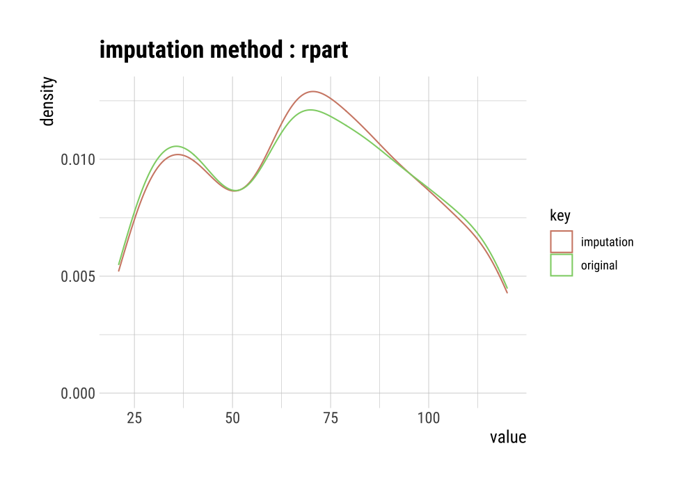

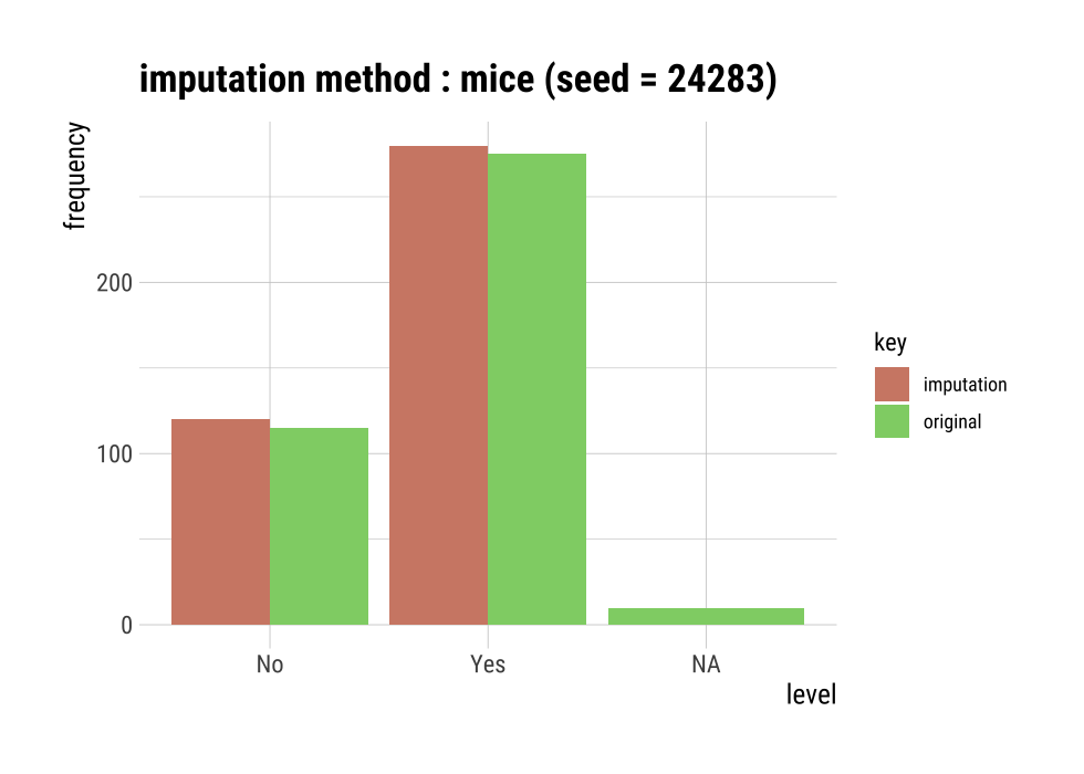
The following imputes the categorical variable urban by the “mice” method.

library(mice)

urban <- imputate_na(carseats, Urban, US, method = "mice")


 iter imp variable
  1   1  Income  Urban
  1   2  Income  Urban
  1   3  Income  Urban
  1   4  Income  Urban
  1   5  Income  Urban
  2   1  Income  Urban
  2   2  Income  Urban
  2   3  Income  Urban
  2   4  Income  Urban
  2   5  Income  Urban
  3   1  Income  Urban
  3   2  Income  Urban
  3   3  Income  Urban
  3   4  Income  Urban
  3   5  Income  Urban
  4   1  Income  Urban
  4   2  Income  Urban
  4   3  Income  Urban
  4   4  Income  Urban
  4   5  Income  Urban
  5   1  Income  Urban
  5   2  Income  Urban
  5   3  Income  Urban
  5   4  Income  Urban
  5   5  Income  Urban


# result of imputation
urban

  [1] Yes Yes Yes Yes Yes No  Yes Yes No  No  No  Yes Yes Yes Yes No 
 [17] Yes Yes No  Yes Yes No  Yes Yes Yes No  No  Yes Yes Yes Yes Yes
 [33] Yes Yes Yes No  No  Yes Yes No  No  Yes Yes Yes Yes Yes No  Yes
 [49] Yes Yes Yes Yes Yes Yes No  Yes Yes Yes Yes Yes Yes No  Yes Yes
 [65] No  No  Yes Yes Yes Yes Yes No  Yes No  No  No  Yes No  Yes Yes
 [81] Yes Yes Yes No  No  No  Yes No  Yes No  No  Yes Yes No  Yes Yes
 [97] No  Yes No  No  No  Yes No  Yes Yes Yes No  Yes Yes No  Yes Yes
[113] Yes Yes Yes Yes No  Yes Yes Yes Yes Yes Yes No  Yes No  Yes Yes
[129] Yes No  Yes Yes Yes Yes Yes No  No  Yes Yes No  Yes Yes Yes Yes
[145] No  Yes Yes No  No  Yes Yes No  No  No  No  Yes Yes No  No  No 
[161] No  No  Yes No  No  Yes Yes Yes Yes Yes Yes Yes Yes Yes No  Yes
[177] No  Yes No  Yes Yes Yes Yes Yes No  Yes No  Yes Yes No  No  Yes
[193] No  Yes Yes Yes Yes Yes Yes Yes No  Yes No  Yes Yes Yes Yes No 
[209] Yes No  No  Yes Yes Yes Yes Yes Yes No  Yes Yes Yes Yes Yes Yes
[225] No  Yes Yes Yes No  No  No  No  Yes No  No  Yes Yes Yes Yes Yes
[241] Yes Yes No  Yes Yes No  Yes Yes Yes Yes Yes Yes Yes No  Yes Yes
[257] Yes Yes No  No  Yes Yes Yes Yes Yes Yes No  No  Yes Yes Yes Yes
[273] Yes Yes Yes Yes Yes Yes No  Yes Yes No  Yes No  No  Yes No  Yes
[289] No  Yes No  No  Yes Yes Yes No  Yes Yes Yes No  Yes Yes Yes Yes
[305] Yes Yes Yes Yes Yes Yes Yes Yes No  Yes Yes Yes Yes No  No  No 
[321] Yes Yes Yes Yes Yes Yes Yes Yes Yes Yes No  Yes Yes Yes Yes Yes
[337] Yes Yes Yes Yes Yes No  No  Yes No  Yes No  No  Yes No  No  No 
[353] Yes No  Yes Yes Yes Yes Yes Yes No  No  Yes Yes Yes No  No  Yes
[369] No  Yes Yes Yes No  Yes Yes Yes Yes No  Yes Yes Yes Yes Yes Yes
[385] Yes Yes Yes No  Yes Yes Yes Yes Yes No  Yes Yes No  Yes Yes Yes
attr(,"var_type")
[1] categorical
attr(,"method")
[1] mice
attr(,"na_pos")
 [1]  33  36  84  94 113 132 151 292 313 339
attr(,"seed")
[1] 24283
attr(,"type")
[1] missing values
attr(,"message")
[1] complete imputation
attr(,"success")
[1] TRUE
Levels: No Yes


# summary of imputation
summary(urban)

* Impute missing values based on Multivariate Imputation by Chained Equations
 - method : mice
 - random seed : 24283

* Information of Imputation (before vs after)
     original imputation original_percent imputation_percent
No        115        120            28.75                 30
Yes       275        280            68.75                 70
<NA>       10          0             2.50                  0


# viz of imputation
plot(urban)

Collaboration with dplyr

The following example imputes the missing value of the Income variable, and then calculates the arithmetic mean for each level of US. In this case, dplyr is used, and it is easily interpreted logically using pipes.

# The mean before and after the imputation of the Income variable
carseats %>%
  mutate(Income_imp = imputate_na(carseats, Income, US, method = "knn")) %>%
  group_by(US) %>%
  summarise(orig = mean(Income, na.rm = TRUE),
            imputation = mean(Income_imp))

# A tibble: 2 x 3
  US     orig imputation
  <fct> <dbl>      <dbl>
1 No     65.8       66.1
2 Yes    70.4       70.5

Imputation of outliers

imputes thr outliers with `imputate_outlier()`

imputate_outlier() imputes the outliers value. The predictor with outliers supports only numeric variables and supports the following methods.

predictor is numerical variable
- “mean” : arithmetic mean
- “median” : median
- “mode” : mode
- “capping” : Impute the upper outliers with 95 percentile, and Impute the bottom outliers with 5 percentile.

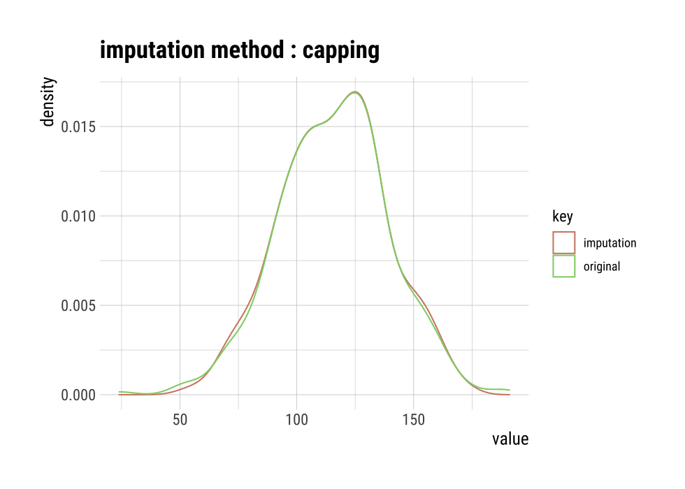
imputate_outlier() imputes the outliers with the numeric variable Price as the “capping” method, as follows. summary() summarizes outliers imputation information, and plot() visualizes imputation information.

price <- imputate_outlier(carseats, Price, method = "capping")

# result of imputation
price

  [1] 120.00  83.00  80.00  97.00 128.00  72.00 108.00 120.00 124.00
 [10] 124.00 100.00  94.00 136.00  86.00 118.00 144.00 110.00 131.00
 [19]  68.00 121.00 131.00 109.00 138.00 109.00 113.00  82.00 131.00
 [28] 107.00  97.00 102.00  89.00 131.00 137.00 128.00 128.00  96.00
 [37] 100.00 110.00 102.00 138.00 126.00 124.00  77.00 134.00  95.00
 [46] 135.00  70.00 108.00  98.00 149.00 108.00 108.00 129.00 119.00
 [55] 144.00 154.00  84.00 117.00 103.00 114.00 123.00 107.00 133.00
 [64] 101.00 104.00 128.00  91.00 115.00 134.00  99.00  99.00 150.00
 [73] 116.00 104.00 136.00  92.00  70.00  89.00 145.00  90.00  79.00
 [82] 128.00 139.00  94.00 121.00 112.00 134.00 126.00 111.00 119.00
 [91] 103.00 107.00 125.00 104.00  84.00 148.00 132.00 129.00 127.00
[100] 107.00 106.00 118.00  97.00  96.00 138.00  97.00 139.00 108.00
[109] 103.00  90.00 116.00 151.00 125.00 127.00 106.00 129.00 128.00
[118] 119.00  99.00 128.00 131.00  87.00 108.00 155.00 120.00  77.00
[127] 133.00 116.00 126.00 147.00  77.00  94.00 136.00  97.00 131.00
[136] 120.00 120.00 118.00 109.00  94.00 129.00 131.00 104.00 159.00
[145] 123.00 117.00 131.00 119.00  97.00  87.00 114.00 103.00 128.00
[154] 150.00 110.00  69.00 157.00  90.00 112.00  70.00 111.00 160.00
[163] 149.00 106.00 141.00 155.05 137.00  93.00 117.00  77.00 118.00
[172]  55.00 110.00 128.00 155.05 122.00 154.00  94.00  81.00 116.00
[181] 149.00  91.00 140.00 102.00  97.00 107.00  86.00  96.00  90.00
[190] 104.00 101.00 173.00  93.00  96.00 128.00 112.00 133.00 138.00
[199] 128.00 126.00 146.00 134.00 130.00 157.00 124.00 132.00 160.00
[208]  97.00  64.00  90.00 123.00 120.00 105.00 139.00 107.00 144.00
[217] 144.00 111.00 120.00 116.00 124.00 107.00 145.00 125.00 141.00
[226]  82.00 122.00 101.00 163.00  72.00 114.00 122.00 105.00 120.00
[235] 129.00 132.00 108.00 135.00 133.00 118.00 121.00  94.00 135.00
[244] 110.00 100.00  88.00  90.00 151.00 101.00 117.00 156.00 132.00
[253] 117.00 122.00 129.00  81.00 144.00 112.00  81.00 100.00 101.00
[262] 118.00 132.00 115.00 159.00 129.00 112.00 112.00 105.00 166.00
[271]  89.00 110.00  63.00  86.00 119.00 132.00 130.00 125.00 151.00
[280] 158.00 145.00 105.00 154.00 117.00  96.00 131.00 113.00  72.00
[289]  97.00 156.00 103.00  89.00  74.00  89.00  99.00 137.00 123.00
[298] 104.00 130.00  96.00  99.00  87.00 110.00  99.00 134.00 132.00
[307] 133.00 120.00 126.00  80.00 166.00 132.00 135.00  54.00 129.00
[316] 171.00  72.00 136.00 130.00 129.00 152.00  98.00 139.00 103.00
[325] 150.00 104.00 122.00 104.00 111.00  89.00 112.00 134.00 104.00
[334] 147.00  83.00 110.00 143.00 102.00 101.00 126.00  91.00  93.00
[343] 118.00 121.00 126.00 149.00 125.00 112.00 107.00  96.00  91.00
[352] 105.00 122.00  92.00 145.00 146.00 164.00  72.00 118.00 130.00
[361] 114.00 104.00 110.00 108.00 131.00 162.00 134.00  77.00  79.00
[370] 122.00 119.00 126.00  98.00 116.00 118.00 124.00  92.00 125.00
[379] 119.00 107.00  89.00 151.00 121.00  68.00 112.00 132.00 160.00
[388] 115.00  78.00 107.00 111.00 124.00 130.00 120.00 139.00 128.00
[397] 120.00 159.00  95.00 120.00
attr(,"method")
[1] "capping"
attr(,"var_type")
[1] "numerical"
attr(,"outlier_pos")
[1]  43 126 166 175 368
attr(,"outliers")
[1]  24  49 191 185  53
attr(,"type")
[1] "outliers"
attr(,"message")
[1] "complete imputation"
attr(,"success")
[1] TRUE
attr(,"class")
[1] "imputation" "numeric"


# summary of imputation
summary(price)

Impute outliers with capping

* Information of Imputation (before vs after)
            Original  Imputation
n        400.0000000 400.0000000
na         0.0000000   0.0000000
mean     115.7950000 115.8927500
sd        23.6766644  22.6109187
se_mean    1.1838332   1.1305459
IQR       31.0000000  31.0000000
skewness  -0.1252862  -0.0461621
kurtosis   0.4518850  -0.3030578
p00       24.0000000  54.0000000
p01       54.9900000  67.9600000
p05       77.0000000  77.0000000
p10       87.0000000  87.0000000
p20       96.8000000  96.8000000
p25      100.0000000 100.0000000
p30      104.0000000 104.0000000
p40      110.0000000 110.0000000
p50      117.0000000 117.0000000
p60      122.0000000 122.0000000
p70      128.3000000 128.3000000
p75      131.0000000 131.0000000
p80      134.0000000 134.0000000
p90      146.0000000 146.0000000
p95      155.0500000 155.0025000
p99      166.0500000 164.0200000
p100     191.0000000 173.0000000


# viz of imputation
plot(price)

Collaboration with dplyr

The following example imputes the outliers of the Price variable, and then calculates the arithmetic mean for each level of US. In this case, dplyr is used, and it is easily interpreted logically using pipes.

# The mean before and after the imputation of the Price variable
carseats %>%
  mutate(Price_imp = imputate_outlier(carseats, Price, method = "capping")) %>%
  group_by(US) %>%
  summarise(orig = mean(Price, na.rm = TRUE),
    imputation = mean(Price_imp, na.rm = TRUE))

# A tibble: 2 x 3
  US     orig imputation
  <fct> <dbl>      <dbl>
1 No     114.       114.
2 Yes    117.       117.

Standardization and Resolving Skewness

Introduction to the use of `transform()`

transform() performs data transformation. Only numeric variables are supported, and the following methods are provided.

Standardization
- “zscore” : z-score transformation. (x - mu) / sigma
- “minmax” : minmax transformation. (x - min) / (max - min)
Resolving Skewness
- “log” : log transformation. log(x)
- “log+1” : log transformation. log(x + 1). Used for values that contain 0.
- “sqrt” : square root transformation.
- “1/x” : 1 / x transformation
- “x^2” : x square transformation
- “x^3” : x^3 square transformation

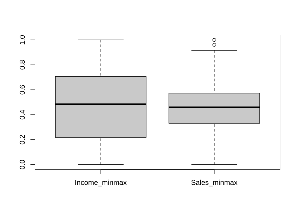
Standardization with `transform()`

Use the methods “zscore” and “minmax” to perform standardization.

carseats %>% 
  mutate(Income_minmax = transform(carseats$Income, method = "minmax"),
    Sales_minmax = transform(carseats$Sales, method = "minmax")) %>% 
  select(Income_minmax, Sales_minmax) %>% 
  boxplot()

Resolving Skewness data with `transform()`

find_skewness() searches for variables with skewed data. This function finds data skewed by search conditions and calculates skewness.

# find index of skewed variables
find_skewness(carseats)

[1] 4


# find names of skewed variables
find_skewness(carseats, index = FALSE)

[1] "Advertising"


# compute the skewness
find_skewness(carseats, value = TRUE)

      Sales   CompPrice      Income Advertising  Population 
      0.185      -0.043       0.045       0.637      -0.051 
      Price         Age   Education 
     -0.125      -0.077       0.044


# compute the skewness & filtering with threshold
find_skewness(carseats, value = TRUE, thres = 0.1)

      Sales Advertising       Price 
      0.185       0.637      -0.125

The skewness of Advertising is 0.637. This means that the distribution of data is somewhat inclined to the left. So, for normal distribution, use transform() to convert to “log” method as follows. summary() summarizes transformation information, and plot() visualizes transformation information.

Advertising_log = transform(carseats$Advertising, method = "log")

# result of transformation
head(Advertising_log)

[1] 2.397895 2.772589 2.302585 1.386294 1.098612 2.564949

# summary of transformation
summary(Advertising_log)

* Resolving Skewness with log

* Information of Transformation (before vs after)
            Original Transformation
n        400.0000000    400.0000000
na         0.0000000      0.0000000
mean       6.6350000           -Inf
sd         6.6503642            NaN
se_mean    0.3325182            NaN
IQR       12.0000000            Inf
skewness   0.6395858            NaN
kurtosis  -0.5451178            NaN
p00        0.0000000           -Inf
p01        0.0000000           -Inf
p05        0.0000000           -Inf
p10        0.0000000           -Inf
p20        0.0000000           -Inf
p25        0.0000000           -Inf
p30        0.0000000           -Inf
p40        2.0000000      0.6931472
p50        5.0000000      1.6094379
p60        8.4000000      2.1265548
p70       11.0000000      2.3978953
p75       12.0000000      2.4849066
p80       13.0000000      2.5649494
p90       16.0000000      2.7725887
p95       19.0000000      2.9444390
p99       23.0100000      3.1359198
p100      29.0000000      3.3672958

# viz of transformation
plot(Advertising_log)

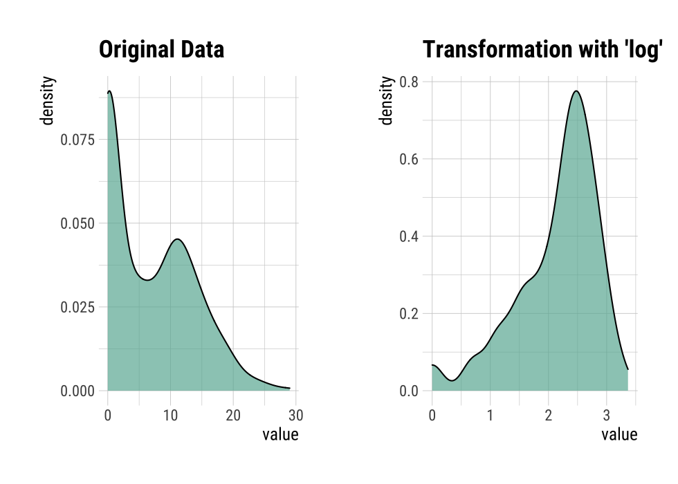
It seems that the raw data contains 0, as there is a -Inf in the log converted value. So this time, convert it to “log+1”.

Advertising_log <- transform(carseats$Advertising, method = "log+1")

# result of transformation
head(Advertising_log)

[1] 2.484907 2.833213 2.397895 1.609438 1.386294 2.639057

# summary of transformation
summary(Advertising_log)

* Resolving Skewness with log+1

* Information of Transformation (before vs after)
            Original Transformation
n        400.0000000   400.00000000
na         0.0000000     0.00000000
mean       6.6350000     1.46247709
sd         6.6503642     1.19436323
se_mean    0.3325182     0.05971816
IQR       12.0000000     2.56494936
skewness   0.6395858    -0.19852549
kurtosis  -0.5451178    -1.66342876
p00        0.0000000     0.00000000
p01        0.0000000     0.00000000
p05        0.0000000     0.00000000
p10        0.0000000     0.00000000
p20        0.0000000     0.00000000
p25        0.0000000     0.00000000
p30        0.0000000     0.00000000
p40        2.0000000     1.09861229
p50        5.0000000     1.79175947
p60        8.4000000     2.23936878
p70       11.0000000     2.48490665
p75       12.0000000     2.56494936
p80       13.0000000     2.63905733
p90       16.0000000     2.83321334
p95       19.0000000     2.99573227
p99       23.0100000     3.17846205
p100      29.0000000     3.40119738

# viz of transformation
# plot(Advertising_log)

Binning

Binning of individual variables using `binning()`

binning() transforms a numeric variable into a categorical variable by binning it. The following types of binning are supported.

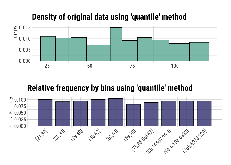
“quantile” : categorize using quantile to include the same frequencies
“equal” : categorize to have equal length segments
“pretty” : categorized into moderately good segments
“kmeans” : categorization using K-means clustering
“bclust” : categorization using bagged clustering technique

Here are some examples of how to bin Income using binning().:

# Binning the carat variable. default type argument is "quantile"
bin <- binning(carseats$Income)
# Print bins class object
bin

binned type: quantile
number of bins: 10
x
        [21,30]         (30,39]         (39,48]         (48,62] 
             40              37              38              40 
        (62,69]         (69,78]   (78,86.56667] (86.56667,96.6] 
             42              33              36              38 
(96.6,108.6333]  (108.6333,120]            <NA> 
             38              38              20

# Summarize bins class object
summary(bin)

            levels freq   rate
1          [21,30]   40 0.1000
2          (30,39]   37 0.0925
3          (39,48]   38 0.0950
4          (48,62]   40 0.1000
5          (62,69]   42 0.1050
6          (69,78]   33 0.0825
7    (78,86.56667]   36 0.0900
8  (86.56667,96.6]   38 0.0950
9  (96.6,108.6333]   38 0.0950
10  (108.6333,120]   38 0.0950
11            <NA>   20 0.0500

# Plot bins class object
plot(bin)

# Using labels argument
bin <- binning(carseats$Income, nbins = 4,
              labels = c("LQ1", "UQ1", "LQ3", "UQ3"))
bin

binned type: quantile
number of bins: 4
x
 LQ1  UQ1  LQ3  UQ3 <NA> 
  95  102   89   94   20

# Using another type argument
binning(carseats$Income, nbins = 5, type = "equal")

binned type: equal
number of bins: 5
x
   [21,40.8]  (40.8,60.6]  (60.6,80.4] (80.4,100.2]  (100.2,120] 
          81           65           94           80           60 
        <NA> 
          20

binning(carseats$Income, nbins = 5, type = "pretty")

binned type: pretty
number of bins: 5
x
  [20,40]   (40,60]   (60,80]  (80,100] (100,120]      <NA> 
       81        65        94        80        60        20


if (requireNamespace("classInt", quietly = TRUE)) {
  binning(carseats$Income, nbins = 5, type = "kmeans")
  binning(carseats$Income, nbins = 5, type = "bclust")
} else {
  cat("If you want to use this feature, you need to install the classInt package.\n")
}

binned type: bclust
number of bins: 5
x
  [21,30.5]   (30.5,49]   (49,75.5] (75.5,97.5]  (97.5,120] 
         40          75         104          86          75 
       <NA> 
         20


# Extract the binned results
extract(bin)

  [1] LQ3  UQ1  LQ1  UQ3  UQ1  UQ3  UQ3  LQ3  UQ3  UQ3  LQ3  UQ3  LQ1 
 [14] LQ1  UQ3  UQ3  <NA> <NA> UQ3  LQ3  LQ3  LQ1  UQ1  LQ1  UQ3  LQ1 
 [27] UQ3  UQ3  LQ3  UQ3  UQ3  UQ1  LQ1  LQ1  UQ1  LQ3  LQ3  LQ1  LQ3 
 [40] <NA> UQ3  UQ1  UQ1  LQ1  LQ3  UQ1  LQ3  UQ3  UQ1  UQ3  LQ1  LQ3 
 [53] LQ1  UQ1  UQ3  LQ3  LQ3  LQ3  UQ3  LQ3  UQ3  LQ1  UQ1  LQ3  UQ1 
 [66] LQ1  UQ3  UQ1  UQ1  UQ1  LQ3  UQ1  UQ1  LQ3  UQ1  UQ3  LQ3  LQ3 
 [79] UQ1  UQ1  UQ3  LQ3  LQ3  LQ1  LQ1  UQ3  LQ3  UQ1  LQ1  UQ1  LQ1 
 [92] UQ1  UQ3  LQ1  <NA> LQ1  LQ1  LQ3  LQ3  UQ1  UQ1  UQ3  LQ1  LQ3 
[105] UQ3  UQ3  LQ1  UQ3  LQ3  UQ1  UQ1  UQ3  UQ3  LQ1  LQ3  <NA> LQ3 
[118] UQ1  LQ3  UQ3  UQ3  LQ3  UQ3  UQ3  UQ3  <NA> UQ1  UQ1  UQ3  UQ3 
[131] LQ3  UQ1  LQ3  UQ3  LQ1  UQ3  LQ3  LQ1  UQ3  UQ1  UQ1  LQ1  LQ3 
[144] LQ3  UQ1  UQ1  LQ3  UQ1  UQ3  UQ3  LQ3  UQ1  LQ3  LQ1  UQ1  LQ3 
[157] LQ1  UQ1  LQ3  UQ1  LQ1  LQ1  <NA> UQ1  UQ1  UQ1  UQ1  LQ3  LQ3 
[170] LQ1  LQ1  UQ3  UQ3  LQ3  LQ1  LQ3  <NA> LQ3  <NA> LQ1  UQ3  LQ3 
[183] UQ1  LQ3  LQ1  UQ3  UQ1  LQ1  LQ1  UQ3  LQ1  LQ1  LQ1  LQ3  UQ3 
[196] UQ3  LQ1  UQ1  LQ3  LQ3  UQ3  LQ3  LQ3  LQ3  LQ3  LQ1  UQ1  UQ3 
[209] <NA> LQ1  LQ1  UQ3  UQ1  LQ3  UQ3  LQ3  <NA> UQ1  UQ1  LQ3  UQ3 
[222] <NA> UQ3  UQ1  LQ3  LQ1  LQ1  UQ1  LQ3  UQ3  UQ1  UQ1  LQ3  LQ3 
[235] UQ1  LQ1  LQ1  LQ1  LQ1  UQ3  LQ3  UQ1  UQ1  LQ1  LQ1  UQ1  UQ1 
[248] UQ3  UQ1  UQ1  UQ3  UQ3  UQ3  LQ1  UQ3  LQ3  LQ1  UQ1  LQ1  LQ1 
[261] UQ3  LQ1  <NA> LQ1  LQ1  LQ1  UQ3  LQ3  UQ1  UQ1  LQ1  UQ1  LQ1 
[274] UQ3  UQ3  UQ3  UQ1  UQ1  UQ3  UQ1  LQ3  UQ1  UQ3  UQ3  UQ1  LQ1 
[287] UQ3  UQ1  LQ1  LQ3  UQ3  LQ3  UQ1  LQ3  LQ3  LQ1  UQ1  LQ3  UQ1 
[300] LQ1  LQ3  UQ3  LQ3  UQ1  UQ3  LQ1  LQ1  UQ3  LQ3  UQ3  UQ1  UQ1 
[313] UQ3  LQ3  <NA> LQ1  LQ1  LQ1  LQ3  UQ1  LQ3  LQ1  UQ1  UQ3  UQ1 
[326] UQ1  LQ1  LQ1  UQ1  UQ1  UQ1  UQ1  LQ1  UQ1  UQ3  LQ3  LQ1  LQ1 
[339] LQ1  UQ1  LQ1  UQ3  UQ3  LQ1  LQ3  UQ1  <NA> LQ1  UQ3  LQ1  <NA>
[352] UQ3  UQ3  UQ1  LQ1  UQ3  UQ3  LQ3  UQ3  UQ1  LQ3  LQ1  UQ1  <NA>
[365] LQ1  LQ1  UQ1  UQ3  LQ1  UQ3  LQ1  LQ3  <NA> <NA> UQ1  UQ1  UQ1 
[378] UQ1  LQ3  UQ3  UQ1  UQ1  LQ1  UQ3  LQ1  LQ3  UQ3  LQ3  LQ3  LQ1 
[391] LQ3  UQ1  LQ1  UQ1  UQ1  UQ3  <NA> LQ1  LQ3  LQ1 
Levels: LQ1 < UQ1 < LQ3 < UQ3


# -------------------------
# Using pipes & dplyr
# -------------------------
library(dplyr)

carseats %>%
 mutate(Income_bin = binning(carseats$Income) %>% 
                     extract()) %>%
 group_by(ShelveLoc, Income_bin) %>%
 summarise(freq = n()) %>%
 arrange(desc(freq)) %>%
 head(10)

# A tibble: 10 x 3
# Groups:   ShelveLoc [1]
  ShelveLoc Income_bin  freq
  <fct>     <ord>      <int>
1 Medium    [21,30]       25
2 Medium    (62,69]       24
3 Medium    (48,62]       23
4 Medium    (39,48]       21
# … with 6 more rows

Optimal Binning with `binning_by()`

binning_by() transforms a numeric variable into a categorical variable by optimal binning. This method is often used when developing a scorecard model.

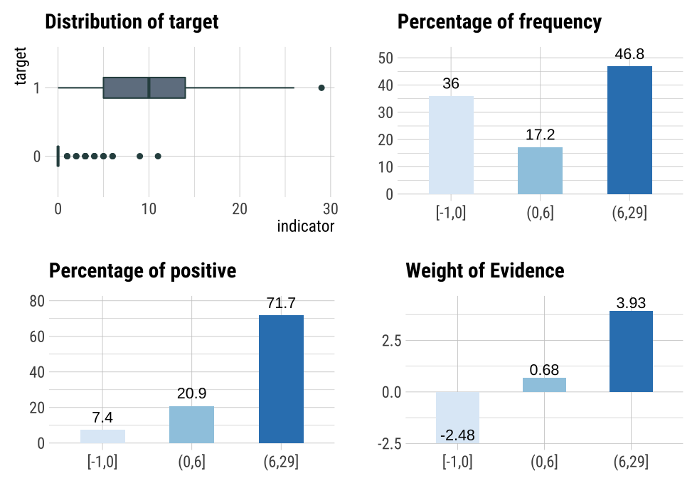
The following binning_by() example optimally binning Advertising considering the target variable US with a binary class.

library(dplyr)

# optimal binning using character
bin <- binning_by(carseats, "US", "Advertising")

# optimal binning using name
bin <- binning_by(carseats, US, Advertising)
bin

binned type: optimal
number of bins: 3
x
[-1,0]  (0,6] (6,29] 
   144     69    187


# summary optimal_bins class
summary(bin)

── Binning Table ──────────────────────── Several Metrics ── 
     Bin CntRec CntPos CntNeg RatePos RateNeg    Odds      WoE
1 [-1,0]    144     19    125 0.07364 0.88028  0.1520 -2.48101
2  (0,6]     69     54     15 0.20930 0.10563  3.6000  0.68380
3 (6,29]    187    185      2 0.71705 0.01408 92.5000  3.93008
4  Total    400    258    142 1.00000 1.00000  1.8169       NA
       IV     JSD     AUC
1 2.00128 0.20093 0.03241
2 0.07089 0.00869 0.01883
3 2.76272 0.21861 0.00903
4 4.83489 0.42823 0.06028

── General Metrics ───────────────────────────────────────── 
• Gini index                       :  -0.87944
• IV (Jeffrey)                     :  4.83489
• JS (Jensen-Shannon) Divergence   :  0.42823
• Kolmogorov-Smirnov Statistics    :  0.80664
• HHI (Herfindahl-Hirschman Index) :  0.37791
• HHI (normalized)                 :  0.06687
• Cramer's V                       :  0.81863 

── Significance Tests ──────────────────── Chisquare Test ── 
   Bin A  Bin B statistics      p_value
1 [-1,0]  (0,6]   87.67064 7.731349e-21
2  (0,6] (6,29]   34.73349 3.780706e-09


# performance table
attr(bin, "performance")

     Bin CntRec CntPos CntNeg CntCumPos CntCumNeg RatePos RateNeg
1 [-1,0]    144     19    125        19       125 0.07364 0.88028
2  (0,6]     69     54     15        73       140 0.20930 0.10563
3 (6,29]    187    185      2       258       142 0.71705 0.01408
4  Total    400    258    142        NA        NA 1.00000 1.00000
  RateCumPos RateCumNeg    Odds   LnOdds      WoE      IV     JSD
1    0.07364    0.88028  0.1520 -1.88387 -2.48101 2.00128 0.20093
2    0.28295    0.98592  3.6000  1.28093  0.68380 0.07089 0.00869
3    1.00000    1.00000 92.5000  4.52721  3.93008 2.76272 0.21861
4         NA         NA  1.8169  0.59713       NA 4.83489 0.42823
      AUC
1 0.03241
2 0.01883
3 0.00903
4 0.06028


# visualize optimal_bins class
plot(bin)


# extract binned results
extract(bin) %>% 
  head(20)

 [1] (6,29] (6,29] (6,29] (0,6]  (0,6]  (6,29] [-1,0] (6,29] [-1,0]
[10] [-1,0] (6,29] (0,6]  (0,6]  (6,29] (6,29] (0,6]  [-1,0] (6,29]
[19] [-1,0] (6,29]
Levels: [-1,0] < (0,6] < (6,29]

Automated report

dlookr provides two automated data transformation reports:

Web page-based dynamic reports can perform in-depth analysis through visualization and statistical tables.
Static reports generated as pdf files or html files can be archived as output of data analysis.

Create a dynamic report using `transformation_web_report()`

transformation_web_report() create dynamic report for object inherited from data.frame(tbl_df, tbl, etc) or data.frame.

Contents of dynamic web report

The contents of the report are as follows.:

Overview
- Data Structures
- Data Types
- Job Informations
Imputation
- Missing Values
- Outliers
Resolving Skewness
Binning
Optimal Binning

Some arguments for dynamic web report

transformation_web_report() generates various reports with the following arguments.

target
- target variable
output_file
- name of generated file.
output_dir
- name of directory to generate report file.
title
- title of report.
subtitle
- subtitle of report.
author
- author of report.
title_color
- color of title.
logo_img
- name of logo image file on top left.
create_date
- The date on which the report is generated.
theme
- name of theme for report. support “orange” and “blue”.
sample_percent
- Sample percent of data for performing data transformation.

The following script creates a data transformation report for the tbl_df class object, heartfailure.

heartfailure %>%
  transformation_web_report(target = "death_event", subtitle = "heartfailure",
                            output_dir = "./", output_file = "transformation.html", 
                            theme = "blue")

Screenshot of dynamic report

The dynamic contents of the report is shown in the following figure.:

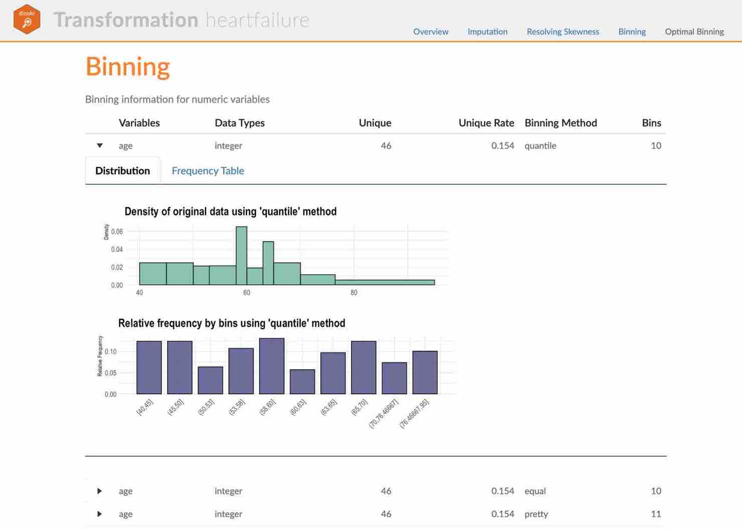
(#fig:trans_web_title)The part of the report

Create a static report using `transformation_paged_report()`

transformation_paged_report() create static report for object inherited from data.frame(tbl_df, tbl, etc) or data.frame.

Contents of static paged report

The contents of the report are as follows.:

Overview
- Data Structures
- Job Informations
Imputation
- Missing Values
- Outliers
Resolving Skewness
Binning
Optimal Binning

Some arguments for static paged report

transformation_paged_report() generates various reports with the following arguments.

target
- target variable
output_format
- report output type. Choose either “pdf” and “html”.
output_file
- name of generated file.
output_dir
- name of directory to generate report file.
title
- title of report.
subtitle
- subtitle of report.
abstract_title
- abstract of report
author
- author of report.
title_color
- color of title.
subtitle_color
- color of subtitle.
logo_img
- name of logo image file on top left.
cover_img
- name of cover image file on center.
create_date
- The date on which the report is generated.
theme
- name of theme for report. support “orange” and “blue”.
sample_percent
- Sample percent of data for performing data tansformation.

The following script creates a data transformation report for the data.frame class object, heartfailure.

heartfailure %>%
  transformation_paged_report(target = "death_event", subtitle = "heartfailure",
                              output_dir = "./", output_file = "transformation.pdf", 
                              theme = "blue")

Screenshot of static report

The cover of the report is shown in the following figure.:

(#fig:trans_paged_cover)The part of the report

The contents of the report is shown in the following figure.:

(#fig:trans_paged_cntent)The dynamic contents of the report

Data Transformation

Preface

datasets

Data Transformation

Imputation of missing values

imputes the missing value with imputate_na()

Collaboration with dplyr

Imputation of outliers

imputes thr outliers with imputate_outlier()

Collaboration with dplyr

Standardization and Resolving Skewness

Introduction to the use of transform()

Standardization with transform()

Resolving Skewness data with transform()

Binning

Binning of individual variables using binning()

Optimal Binning with binning_by()

Automated report

Create a dynamic report using transformation_web_report()

Contents of dynamic web report

Some arguments for dynamic web report

Screenshot of dynamic report

Create a static report using transformation_paged_report()

Contents of static paged report

Some arguments for static paged report

Screenshot of static report

imputes the missing value with `imputate_na()`

imputes thr outliers with `imputate_outlier()`

Introduction to the use of `transform()`

Standardization with `transform()`

Resolving Skewness data with `transform()`

Binning of individual variables using `binning()`

Optimal Binning with `binning_by()`

Create a dynamic report using `transformation_web_report()`

Create a static report using `transformation_paged_report()`