alookr vignettes: Classification Modeling

Preface

Once the data set is ready for model development, the model is fitted, predicted and evaluated in the following ways:

Cleansing the dataset
Split the data into a train set and a test set
Modeling and Evaluate, Predict
- Modeling
  - Binary classification modeling
- Evaluate the model
  - Predict test set using fitted model
  - Calculate the performance metric
  - Plot the ROC curve
  - Tunning the cut-off
- Predict
  - Predict
  - Predict with cut-off

The alookr package makes these steps fast and easy:

Data: Wisconsin Breast Cancer Data

BreastCancer of mlbench package is a breast cancer data. The objective is to identify each of a number of benign or malignant classes.

A data frame with 699 observations on 11 variables, one being a character variable, 9 being ordered or nominal, and 1 target class.:

Id : character. Sample code number
Cl.thickness : ordered factor. Clump Thickness
Cell.size : ordered factor. Uniformity of Cell Size
Cell.shape : ordered factor. Uniformity of Cell Shape
Marg.adhesion : ordered factor. Marginal Adhesion
Epith.c.size : ordered factor. Single Epithelial Cell Size
Bare.nuclei : factor. Bare Nuclei
Bl.cromatin : factor. Bland Chromatin
Normal.nucleoli : factor. Normal Nucleoli
Mitoses : factor. Mitoses
Class : factor. Class. level is benign and malignant.

library(mlbench)
data(BreastCancer)

# class of each variables
sapply(BreastCancer, function(x) class(x)[1])

             Id    Cl.thickness       Cell.size      Cell.shape 
    "character"       "ordered"       "ordered"       "ordered" 
  Marg.adhesion    Epith.c.size     Bare.nuclei     Bl.cromatin 
      "ordered"       "ordered"        "factor"        "factor" 
Normal.nucleoli         Mitoses           Class 
       "factor"        "factor"        "factor"

Preperation the data

Perform data preprocessing as follows.:

Find and imputate variables that contain missing values.
Split the data into a train set and a test set.
To solve the imbalanced class, perform sampling in the train set of raw data.
Cleansing the dataset for classification modeling.

Fix the missing value with `dlookr::imputate_na()`

find the variables that include missing value. and imputate the missing value using imputate_na() in dlookr package.

library(dlookr)
library(dplyr)

# variable that have a missing value
diagnose(BreastCancer) %>%
  filter(missing_count > 0)

# A tibble: 1 x 6
  variables   types  missing_count missing_percent unique_count
  <chr>       <chr>          <int>           <dbl>        <int>
1 Bare.nuclei factor            16            2.29           11
# … with 1 more variable: unique_rate <dbl>


# imputation of missing value
breastCancer <- BreastCancer %>%
  mutate(Bare.nuclei = imputate_na(BreastCancer, Bare.nuclei, Class,
                         method = "mice", no_attrs = TRUE, print_flag = FALSE))

Split data set

Splits the dataset into a train set and a test set with `split_by()`

split_by() in the alookr package splits the dataset into a train set and a test set.

The ratio argument of the split_by() function specifies the ratio of the train set.

split_by() creates a class object named split_df.

library(alookr)

# split the data into a train set and a test set by default arguments
sb <- breastCancer %>%
  split_by(target = Class)

# show the class name
class(sb)

[1] "split_df"   "grouped_df" "tbl_df"     "tbl"        "data.frame"


# split the data into a train set and a test set by ratio = 0.6
tmp <- breastCancer %>%
  split_by(Class, ratio = 0.6)

The summary() function displays the following useful information about the split_df object:

random seed : The random seed is the random seed used internally to separate the data
split data : Information of splited data
- train set count : number of train set
- test set count : number of test set
target variable : Target variable name
- minority class : name and ratio(In parentheses) of minority class
- majority class : name and ratio(In parentheses) of majority class

# summary() display the some information
summary(sb)

** Split train/test set information **
 + random seed        :  90170 
 + split data            
    - train set count :  489 
    - test set count  :  210 
 + target variable    :  Class 
    - minority class  :  malignant (0.344778)
    - majority class  :  benign (0.655222)


# summary() display the some information
summary(tmp)

** Split train/test set information **
 + random seed        :  85477 
 + split data            
    - train set count :  419 
    - test set count  :  280 
 + target variable    :  Class 
    - minority class  :  malignant (0.344778)
    - majority class  :  benign (0.655222)

Check missing levels in the train set

In the case of categorical variables, when a train set and a test set are separated, a specific level may be missing from the train set.

In this case, there is no problem when fitting the model, but an error occurs when predicting with the model you created. Therefore, preprocessing is performed to avoid missing data preprocessing.

In the following example, fortunately, there is no categorical variable that contains the missing levels in the train set.

# list of categorical variables in the train set that contain missing levels
nolevel_in_train <- sb %>%
  compare_target_category() %>% 
  filter(is.na(train)) %>% 
  select(variable) %>% 
  unique() %>% 
  pull

nolevel_in_train

character(0)


# if any of the categorical variables in the train set contain a missing level, 
# split them again.
while (length(nolevel_in_train) > 0) {
  sb <- breastCancer %>%
    split_by(Class)

  nolevel_in_train <- sb %>%
    compare_target_category() %>% 
    filter(is.na(train)) %>% 
    select(variable) %>% 
    unique() %>% 
    pull
}

Handling the imbalanced classes data with `sampling_target()`

Issue of imbalanced classes data

Imbalanced classes(levels) data means that the number of one level of the frequency of the target variable is relatively small. In general, the proportion of positive classes is relatively small. For example, in the model of predicting spam, the class of interest spam is less than non-spam.

Imbalanced classes data is a common problem in machine learning classification.

table() and prop.table() are traditionally useful functions for diagnosing imbalanced classes data. However, alookr’s summary() is simpler and provides more information.

# train set frequency table - imbalanced classes data
table(sb$Class)


   benign malignant 
      458       241


# train set relative frequency table - imbalanced classes data
prop.table(table(sb$Class))


   benign malignant 
0.6552217 0.3447783


# using summary function - imbalanced classes data
summary(sb)

** Split train/test set information **
 + random seed        :  90170 
 + split data            
    - train set count :  489 
    - test set count  :  210 
 + target variable    :  Class 
    - minority class  :  malignant (0.344778)
    - majority class  :  benign (0.655222)

Handling the imbalanced classes data

Most machine learning algorithms work best when the number of samples in each class are about equal. And most algorithms are designed to maximize accuracy and reduce error. So, we requre handling an imbalanced class problem.

sampling_target() performs sampling to solve an imbalanced classes data problem.

Resampling - oversample minority class

Oversampling can be defined as adding more copies of the minority class.

Oversampling is performed by specifying “ubOver” in the method argument of the sampling_target() function.

# to balanced by over sampling
train_over <- sb %>%
  sampling_target(method = "ubOver")

# frequency table 
table(train_over$Class)


   benign malignant 
      318       318

Resampling - undersample majority class

Undersampling can be defined as removing some observations of the majority class.

Undersampling is performed by specifying “ubUnder” in the method argument of the sampling_target() function.

# to balanced by under sampling
train_under <- sb %>%
  sampling_target(method = "ubUnder")

# frequency table 
table(train_under$Class)


   benign malignant 
      171       171

Generate synthetic samples - SMOTE

SMOTE(Synthetic Minority Oversampling Technique) uses a nearest neighbors algorithm to generate new and synthetic data.

SMOTE is performed by specifying “ubSMOTE” in the method argument of the sampling_target() function.

# to balanced by SMOTE
train_smote <- sb %>%
  sampling_target(seed = 1234L, method = "ubSMOTE")

# frequency table 
table(train_smote$Class)


   benign malignant 
      684       513

Cleansing the dataset for classification modeling with `cleanse()`

The cleanse() cleanse the dataset for classification modeling.

This function is useful when fit the classification model. This function does the following.:

Remove the variable with only one value.
And remove variables that have a unique number of values relative to the number of observations for a character or categorical variable.
- In this case, it is a variable that corresponds to an identifier or an identifier.
And converts the character to factor.

In this example, The cleanse() function removed a variable ID with a high unique rate.

# clean the training set
train <- train_smote %>%
  cleanse

── Checking unique value ─────────────────────────── unique value is one ──
No variables that unique value is one.

── Checking unique rate ─────────────────────────────── high unique rate ──
• Id = 424(0.35421888053467)

── Checking character variables ─────────────────────── categorical data ──
No character variables.

Extract test set for evaluation of the model with `extract_set()`

# extract test set
test <- sb %>%
  extract_set(set = "test")

Binary classification modeling with `run_models()`

run_models() performs some representative binary classification modeling using split_df object created by split_by().

run_models() executes the process in parallel when fitting the model. However, it is not supported in MS-Windows operating system and RStudio environment.

Currently supported algorithms are as follows.:

logistic : logistic regression using stats package
rpart : Recursive Partitioning Trees using rpart package
ctree : Conditional Inference Trees using party package
randomForest :Classification with Random Forest using randomForest package
ranger : A Fast Implementation of Random Forests using ranger package
xgboost : Extreme Gradient Boosting using xgboost package

run_models() returns a model_df class object.

The model_df class object contains the following variables.:

step : character. The current stage in the classification modeling process.
- For objects created with run_models(), the value of the variable is “1.Fitted”.
model_id : model identifiers
target : name of target variable
positive : positive class in target variable
fitted_model : list. Fitted model object by model_id’s algorithms

result <- train %>% 
  run_models(target = "Class", positive = "malignant")
result

# A tibble: 7 x 7
  step     model_id    target is_factor positive negative fitted_model
  <chr>    <chr>       <chr>  <lgl>     <chr>    <chr>    <list>      
1 1.Fitted logistic    Class  TRUE      maligna… benign   <glm>       
2 1.Fitted rpart       Class  TRUE      maligna… benign   <rpart>     
3 1.Fitted ctree       Class  TRUE      maligna… benign   <BinaryTr>  
4 1.Fitted randomFore… Class  TRUE      maligna… benign   <rndmFrs.>  
5 1.Fitted ranger      Class  TRUE      maligna… benign   <ranger>    
6 1.Fitted xgboost     Class  TRUE      maligna… benign   <xgb.Bstr>  
# … with 1 more row

Evaluate the model

Evaluate the predictive performance of fitted models.

Predict test set using fitted model with `run_predict()`

run_predict() predict the test set using model_df class fitted by run_models().

run_predict () is executed in parallel when predicting by model. However, it is not supported in MS-Windows operating system and RStudio environment.

The model_df class object contains the following variables.:

step : character. The current stage in the classification modeling process.
- For objects created with run_predict(), the value of the variable is “2.Predicted”.
model_id : character. Type of fit model.
target : character. Name of target variable.
positive : character. Level of positive class of binary classification.
fitted_model : list. Fitted model object by model_id’s algorithms.
predicted : result of predcit by each models

pred <- result %>%
  run_predict(test)
pred

# A tibble: 7 x 8
  step      model_id   target is_factor positive negative fitted_model
  <chr>     <chr>      <chr>  <lgl>     <chr>    <chr>    <list>      
1 2.Predic… logistic   Class  TRUE      maligna… benign   <glm>       
2 2.Predic… rpart      Class  TRUE      maligna… benign   <rpart>     
3 2.Predic… ctree      Class  TRUE      maligna… benign   <BinaryTr>  
4 2.Predic… randomFor… Class  TRUE      maligna… benign   <rndmFrs.>  
5 2.Predic… ranger     Class  TRUE      maligna… benign   <ranger>    
6 2.Predic… xgboost    Class  TRUE      maligna… benign   <xgb.Bstr>  
# … with 1 more row, and 1 more variable: predicted <list>

Calculate the performance metric with `run_performance()`

run_performance() calculate the performance metric of model_df class predicted by run_predict().

run_performance () is performed in parallel when calculating the performance evaluation metrics However, it is not supported in MS-Windows operating system and RStudio environment.

The model_df class object contains the following variables.:

step : character. The current stage in the classification modeling process.
- For objects created with run_performance(), the value of the variable is “3.Performanced”.
model_id : character. Type of fit model.
target : character. Name of target variable.
positive : character. Level of positive class of binary classification.
fitted_model : list. Fitted model object by model_id’s algorithms
predicted : list. Predicted value by individual model. Each value has a predict_class class object.
performance : list. Calculate metrics by individual model. Each value has a numeric vector.

# Calculate performace metrics.
perf <- run_performance(pred)
perf

# A tibble: 7 x 7
  step    model_id  target positive fitted_model predicted performance
  <chr>   <chr>     <chr>  <chr>    <list>       <list>    <list>     
1 3.Perf… logistic  Class  maligna… <glm>        <fct [21… <dbl [15]> 
2 3.Perf… rpart     Class  maligna… <rpart>      <fct [21… <dbl [15]> 
3 3.Perf… ctree     Class  maligna… <BinaryTr>   <fct [21… <dbl [15]> 
4 3.Perf… randomFo… Class  maligna… <rndmFrs.>   <fct [21… <dbl [15]> 
5 3.Perf… ranger    Class  maligna… <ranger>     <fct [21… <dbl [15]> 
6 3.Perf… xgboost   Class  maligna… <xgb.Bstr>   <fct [21… <dbl [15]> 
# … with 1 more row

The performance variable contains a list object, which contains 15 performance metrics:

ZeroOneLoss : Normalized Zero-One Loss(Classification Error Loss).
Accuracy : Accuracy.
Precision : Precision.
Recall : Recall.
Sensitivity : Sensitivity.
Specificity : Specificity.
F1_Score : F1 Score.
Fbeta_Score : F-Beta Score.
LogLoss : Log loss / Cross-Entropy Loss.
AUC : Area Under the Receiver Operating Characteristic Curve (ROC AUC).
Gini : Gini Coefficient.
PRAUC : Area Under the Precision-Recall Curve (PR AUC).
LiftAUC : Area Under the Lift Chart.
GainAUC : Area Under the Gain Chart.
KS_Stat : Kolmogorov-Smirnov Statistic.

# Performance by analytics models
performance <- perf$performance
names(performance) <- perf$model_id
performance

$logistic
ZeroOneLoss    Accuracy   Precision      Recall Sensitivity 
 0.06666667  0.93333333  0.90000000  0.90000000  0.90000000 
Specificity    F1_Score Fbeta_Score     LogLoss         AUC 
 0.95000000  0.90000000  0.90000000  2.23608577  0.93147959 
       Gini       PRAUC     LiftAUC     GainAUC     KS_Stat 
 0.85918367  0.06524816  1.23041695  0.78765306 86.42857143 

$rpart
ZeroOneLoss    Accuracy   Precision      Recall Sensitivity 
 0.04761905  0.95238095  0.89473684  0.97142857  0.97142857 
Specificity    F1_Score Fbeta_Score     LogLoss         AUC 
 0.94285714  0.93150685  0.93150685  0.47177933  0.96418367 
       Gini       PRAUC     LiftAUC     GainAUC     KS_Stat 
 0.93836735  0.68264643  1.88355147  0.80945578 92.14285714 

$ctree
ZeroOneLoss    Accuracy   Precision      Recall Sensitivity 
 0.05238095  0.94761905  0.88311688  0.97142857  0.97142857 
Specificity    F1_Score Fbeta_Score     LogLoss         AUC 
 0.93571429  0.92517007  0.92517007  0.41646571  0.98056122 
       Gini       PRAUC     LiftAUC     GainAUC     KS_Stat 
 0.96163265  0.79154066  1.99494847  0.82037415 91.42857143 

$randomForest
ZeroOneLoss    Accuracy   Precision      Recall Sensitivity 
 0.01904762  0.98095238  0.94594595  1.00000000  1.00000000 
Specificity    F1_Score Fbeta_Score     LogLoss         AUC 
 0.97142857  0.97222222  0.97222222  0.07998188  0.99500000 
       Gini       PRAUC     LiftAUC     GainAUC     KS_Stat 
 0.99000000  0.88843776  2.03490054  0.83000000 97.14285714 

$ranger
ZeroOneLoss    Accuracy   Precision      Recall Sensitivity 
 0.02857143  0.97142857  0.92105263  1.00000000  1.00000000 
Specificity    F1_Score Fbeta_Score     LogLoss         AUC 
 0.95714286  0.95890411  0.95890411  0.07413234  0.99673469 
       Gini       PRAUC     LiftAUC     GainAUC     KS_Stat 
 0.99346939  0.90723276  2.03167355  0.83115646 97.14285714 

$xgboost
ZeroOneLoss    Accuracy   Precision      Recall Sensitivity 
 0.02857143  0.97142857  0.93243243  0.98571429  0.98571429 
Specificity    F1_Score Fbeta_Score     LogLoss         AUC 
 0.96428571  0.95833333  0.95833333  0.09591749  0.99489796 
       Gini       PRAUC     LiftAUC     GainAUC     KS_Stat 
 0.98959184  0.94665981  2.09969906  0.82993197 95.00000000 

$lasso
ZeroOneLoss    Accuracy   Precision      Recall Sensitivity 
 0.02857143  0.97142857  0.95714286  0.95714286  0.95714286 
Specificity    F1_Score Fbeta_Score     LogLoss         AUC 
 0.97857143  0.95714286  0.95714286  0.05848341  0.99816327 
       Gini       PRAUC     LiftAUC     GainAUC     KS_Stat 
 0.99632653  0.98201545  2.08070669  0.83210884 97.14285714

If you change the list object to tidy format, you’ll see the following at a glance:

# Convert to matrix for compare performace.
sapply(performance, "c")

               logistic       rpart       ctree randomForest
ZeroOneLoss  0.06666667  0.04761905  0.05238095   0.01904762
Accuracy     0.93333333  0.95238095  0.94761905   0.98095238
Precision    0.90000000  0.89473684  0.88311688   0.94594595
Recall       0.90000000  0.97142857  0.97142857   1.00000000
Sensitivity  0.90000000  0.97142857  0.97142857   1.00000000
Specificity  0.95000000  0.94285714  0.93571429   0.97142857
F1_Score     0.90000000  0.93150685  0.92517007   0.97222222
Fbeta_Score  0.90000000  0.93150685  0.92517007   0.97222222
LogLoss      2.23608577  0.47177933  0.41646571   0.07998188
AUC          0.93147959  0.96418367  0.98056122   0.99500000
Gini         0.85918367  0.93836735  0.96163265   0.99000000
PRAUC        0.06524816  0.68264643  0.79154066   0.88843776
LiftAUC      1.23041695  1.88355147  1.99494847   2.03490054
GainAUC      0.78765306  0.80945578  0.82037415   0.83000000
KS_Stat     86.42857143 92.14285714 91.42857143  97.14285714
                 ranger     xgboost       lasso
ZeroOneLoss  0.02857143  0.02857143  0.02857143
Accuracy     0.97142857  0.97142857  0.97142857
Precision    0.92105263  0.93243243  0.95714286
Recall       1.00000000  0.98571429  0.95714286
Sensitivity  1.00000000  0.98571429  0.95714286
Specificity  0.95714286  0.96428571  0.97857143
F1_Score     0.95890411  0.95833333  0.95714286
Fbeta_Score  0.95890411  0.95833333  0.95714286
LogLoss      0.07413234  0.09591749  0.05848341
AUC          0.99673469  0.99489796  0.99816327
Gini         0.99346939  0.98959184  0.99632653
PRAUC        0.90723276  0.94665981  0.98201545
LiftAUC      2.03167355  2.09969906  2.08070669
GainAUC      0.83115646  0.82993197  0.83210884
KS_Stat     97.14285714 95.00000000 97.14285714

compare_performance() return a list object(results of compared model performance). and list has the following components:

recommend_model : character. The name of the model that is recommended as the best among the various models.
top_count : numeric. The number of best performing performance metrics by model.
mean_rank : numeric. Average of ranking individual performance metrics by model.
top_metric : list. The name of the performance metric with the best performance on individual performance metrics by model.

In this example, compare_performance() recommend the “ranger” model.

# Compaire the Performance metrics of each model
comp_perf <- compare_performance(pred)
comp_perf

$recommend_model
[1] "lasso"

$top_metric_count
    logistic        rpart        ctree randomForest       ranger 
           0            0            0            4            2 
     xgboost        lasso 
           1            7 

$mean_rank
    logistic        rpart        ctree randomForest       ranger 
    6.692308     5.576923     5.576923     2.307692     2.576923 
     xgboost        lasso 
    3.153846     2.115385 

$top_metric
$top_metric$logistic
NULL

$top_metric$rpart
NULL

$top_metric$ctree
NULL

$top_metric$randomForest
[1] "ZeroOneLoss" "Accuracy"    "Recall"      "F1_Score"   

$top_metric$ranger
[1] "Recall"  "KS_Stat"

$top_metric$xgboost
[1] "LiftAUC"

$top_metric$lasso
[1] "Precision"   "Specificity" "LogLoss"     "AUC"        
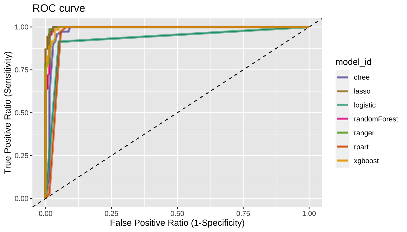
[5] "Gini"        "PRAUC"       "GainAUC"

Plot the ROC curve with `plot_performance()`

compare_performance() plot ROC curve.

# Plot ROC curve
plot_performance(pred)

Tunning the cut-off

In general, if the prediction probability is greater than 0.5 in the binary classification model, it is predicted as positive class. In other words, 0.5 is used for the cut-off value. This applies to most model algorithms. However, in some cases, the performance can be tuned by changing the cut-off value.

plot_cutoff () visualizes a plot to select the cut-off value, and returns the cut-off value.

pred_best <- pred %>% 
  filter(model_id == comp_perf$recommend_model) %>% 
  select(predicted) %>% 
  pull %>% 
  .[[1]] %>% 
  attr("pred_prob")

cutoff <- plot_cutoff(pred_best, test$Class, "malignant", type = "mcc")

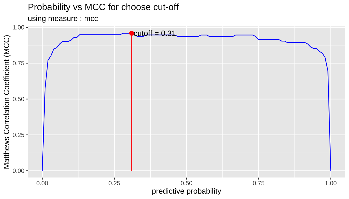
cutoff

[1] 0.31


cutoff2 <- plot_cutoff(pred_best, test$Class, "malignant", type = "density")

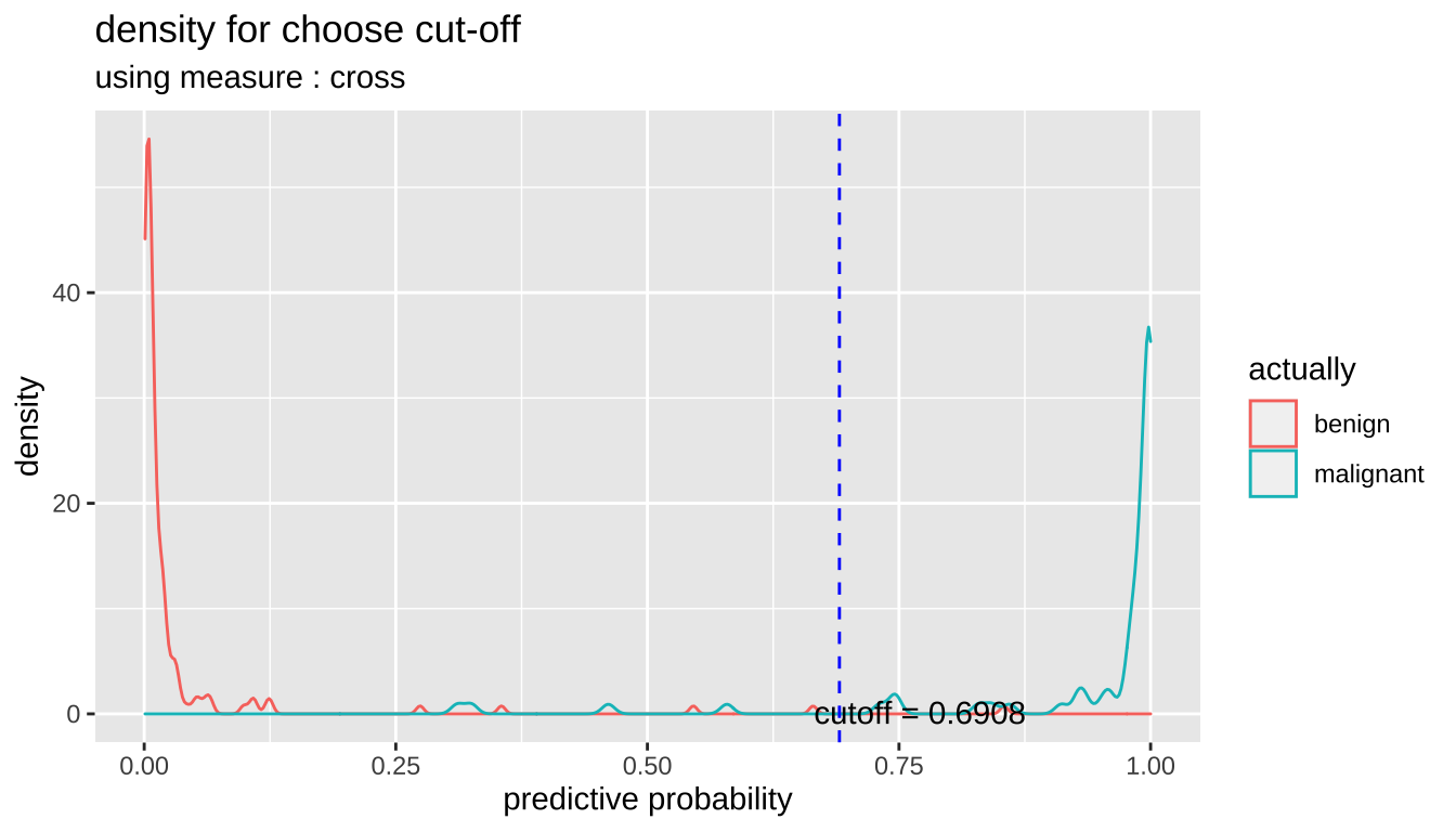
cutoff2

[1] 0.6908


cutoff3 <- plot_cutoff(pred_best, test$Class, "malignant", type = "prob")

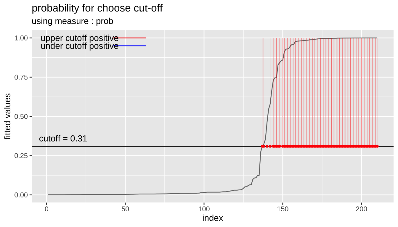
cutoff3

[1] 0.31

Performance comparison between prediction and tuned cut-off with `performance_metric()`

Compare the performance of the original prediction with that of the tuned cut-off. Compare the cut-off with the non-cut model for the model with the best performance comp_perf$recommend_model.

comp_perf$recommend_model

[1] "lasso"


# extract predicted probability
idx <- which(pred$model_id == comp_perf$recommend_model)
pred_prob <- attr(pred$predicted[[idx]], "pred_prob")

# or, extract predicted probability using dplyr
pred_prob <- pred %>% 
  filter(model_id == comp_perf$recommend_model) %>% 
  select(predicted) %>% 
  pull %>% 
  "[["(1) %>% 
  attr("pred_prob")

# predicted probability
pred_prob

  [1] 0.0174789286 0.0519610507 0.0032789015 0.0175209919 0.0032869065
  [6] 0.0064426070 0.0061333348 0.3549603767 0.9816825081 0.8597953337
 [11] 0.9586400416 0.9829636303 0.9807564163 0.8423412779 0.5789667959
 [16] 0.0018752648 0.0174789286 0.0198675394 0.9962768052 0.0343359964
 [21] 0.1091094158 0.9998443243 0.9999145915 0.0174789286 0.0036986645
 [26] 0.0032789015 0.9999991641 0.9963338820 0.0640467480 0.9998845141
 [31] 0.9999213746 0.0018752648 0.9996409596 0.0100335360 0.9295070011
 [36] 0.0062525812 0.0198675394 0.9981252268 0.0015038391 0.0018798495
 [41] 0.9855421605 0.0029222429 0.4612051835 0.2741038918 0.0026301961
 [46] 0.0989389839 0.0254864819 0.9881447326 0.9962328663 0.0057410803
 [51] 0.9932372955 0.0174789286 0.0519610507 0.9882845720 0.0046075035
 [56] 0.9112488848 0.0049576630 0.0174789286 0.0423490116 0.0010718527
 [61] 0.0057550617 0.0302801908 0.9999561536 0.9993322438 0.0032789015
 [66] 0.9999961972 0.9991843932 0.0036806781 0.9968751445 0.0026301961
 [71] 0.9799969986 0.6646602131 0.9880154141 0.0155439828 0.9987995118
 [76] 0.0015219772 0.9996213115 0.9990884566 0.9992499097 0.9980651483
 [81] 0.7459408405 0.0032789015 0.7459408405 0.0114572781 0.0065363079
 [86] 0.0032789015 0.9999947042 0.7308047117 0.0010718527 0.9906787589
 [91] 0.0032789015 0.0032789015 0.9349685763 0.0032789015 0.9994083226
 [96] 0.0040969162 0.0015038391 0.0063453940 0.8544840270 0.8291636536
[101] 0.0032789015 0.0106386198 0.0594483184 0.0315084513 0.9794110022
[106] 0.0032789015 0.9600304045 0.9946262997 0.9999201601 0.0010718527
[111] 0.9999965110 0.0012181350 0.0017089763 0.9996232840 0.0057690770
[116] 0.0087428342 0.0069747680 0.0142279160 0.1077781495 0.9992975276
[121] 0.0018752648 0.0654855639 0.9774531461 0.0082488763 0.0013775228
[126] 0.0018798495 0.9988106910 0.0101668011 0.0041516620 0.9976670706
[131] 0.9996056910 0.0107418740 0.0089487465 0.0065917287 0.0141284785
[136] 0.0032949311 0.0061482656 0.0057690770 0.9925235631 0.0080984931
[141] 0.3111760831 0.3249935903 0.9841031438 0.0008594184 0.0076723952
[146] 0.0100578652 0.0174789286 0.0058351459 0.0022745826 0.0010718527
[151] 0.0015038391 0.0039423091 0.0013367271 0.0071863706 0.0174789286
[156] 0.0223098968 0.0080788648 0.0057550617 0.0322182336 0.0100578652
[161] 0.0303521088 0.9994192211 0.0015075171 0.9970521458 0.1240980381
[166] 0.1239033127 0.0175209919 0.0302801908 0.0032789015 0.0057550617
[171] 0.0106900042 0.0165141914 0.9975221618 0.0018752648 0.0186581120
[176] 0.0107418740 0.9515212505 0.0100822529 0.9988956651 0.9999999199
[181] 0.0026366216 0.0100578652 0.5456300156 0.0010718527 0.0051179763
[186] 0.0263618680 0.0010718527 0.9999789834 0.0057550617 0.0015219772
[191] 0.0013513340 0.0199857423 0.0057550617 0.0010718527 0.0018752648
[196] 0.0021309597 0.9963922021 0.0057410803 0.0234847484 0.0018752648
[201] 0.0100822529 0.0010718527 0.0010718527 0.0010718527 0.0057690770
[206] 0.9286862826 0.0032949311 0.0115808996 0.9980659398 0.9854399625


# compaire Accuracy
performance_metric(pred_prob, test$Class, "malignant", "Accuracy")

[1] 0.9714286

performance_metric(pred_prob, test$Class, "malignant", "Accuracy",
                   cutoff = cutoff)

[1] 0.9809524


# compaire Confusion Matrix
performance_metric(pred_prob, test$Class, "malignant", "ConfusionMatrix")

           actual
predict     benign malignant
  benign       137         3
  malignant      3        67

performance_metric(pred_prob, test$Class, "malignant", "ConfusionMatrix", 
                   cutoff = cutoff)

           actual
predict     benign malignant
  benign       136         0
  malignant      4        70


# compaire F1 Score
performance_metric(pred_prob, test$Class, "malignant", "F1_Score")

[1] 0.9571429

performance_metric(pred_prob, test$Class,  "malignant", "F1_Score", 
                   cutoff = cutoff)

[1] 0.9722222

performance_metric(pred_prob, test$Class,  "malignant", "F1_Score", 
                   cutoff = cutoff2)

[1] 0.9635036

If the performance of the tuned cut-off is good, use it as a cut-off to predict positives.

Predict

If you have selected a good model from several models, then perform the prediction with that model.

Create data set for predict

Create sample data for predicting by extracting 100 samples from the data set used in the previous under sampling example.

data_pred <- train_under %>% 
  cleanse

── Checking unique value ─────────────────────────── unique value is one ──
No variables that unique value is one.

── Checking unique rate ─────────────────────────────── high unique rate ──
• Id = 336(0.982456140350877)

── Checking character variables ─────────────────────── categorical data ──
No character variables.


set.seed(1234L)
data_pred <- data_pred %>% 
  nrow %>% 
  seq %>% 
  sample(size = 50) %>% 
  data_pred[., ]

Predict with alookr and dplyr

Do a predict using the dplyr package. The last factor() function eliminates unnecessary information.

pred_actual <- pred %>%
  filter(model_id == comp_perf$recommend_model) %>% 
  run_predict(data_pred) %>% 
  select(predicted) %>% 
  pull %>% 
  "[["(1) %>% 
  factor()

pred_actual

 [1] benign    benign    benign    malignant malignant benign   
 [7] malignant benign    benign    benign    benign    benign   
[13] benign    benign    malignant benign    malignant malignant
[19] malignant benign    malignant benign    benign    malignant
[25] benign    malignant malignant benign    benign    malignant
[31] malignant malignant benign    malignant malignant benign   
[37] malignant benign    malignant malignant malignant malignant
[43] benign    benign    benign    malignant benign    benign   
[49] malignant malignant
Levels: benign malignant

If you want to predict by cut-off, specify the cutoff argument in the run_predict() function as follows.:

In the example, there is no difference between the results of using cut-off and not.

pred_actual2 <- pred %>%
  filter(model_id == comp_perf$recommend_model) %>% 
  run_predict(data_pred, cutoff) %>% 
  select(predicted) %>% 
  pull %>% 
  "[["(1) %>% 
  factor()

pred_actual2

 [1] benign    benign    benign    malignant malignant benign   
 [7] malignant benign    benign    benign    benign    benign   
[13] benign    benign    malignant benign    malignant malignant
[19] malignant benign    malignant benign    benign    malignant
[25] benign    malignant malignant benign    benign    malignant
[31] malignant malignant benign    malignant malignant benign   
[37] malignant benign    malignant malignant malignant malignant
[43] benign    benign    benign    malignant benign    malignant
[49] malignant malignant
Levels: benign malignant


sum(pred_actual != pred_actual2)

[1] 1

Classification Modeling

Preface

Data: Wisconsin Breast Cancer Data

Preperation the data

Fix the missing value with dlookr::imputate_na()

Split data set

Splits the dataset into a train set and a test set with split_by()

Check missing levels in the train set

Handling the imbalanced classes data with sampling_target()

Issue of imbalanced classes data

Handling the imbalanced classes data

Resampling - oversample minority class

Resampling - undersample majority class

Generate synthetic samples - SMOTE

Cleansing the dataset for classification modeling with cleanse()

Extract test set for evaluation of the model with extract_set()

Binary classification modeling with run_models()

Evaluate the model

Predict test set using fitted model with run_predict()

Calculate the performance metric with run_performance()

Plot the ROC curve with plot_performance()

Tunning the cut-off

Performance comparison between prediction and tuned cut-off with performance_metric()

Predict

Create data set for predict

Predict with alookr and dplyr

Fix the missing value with `dlookr::imputate_na()`

Splits the dataset into a train set and a test set with `split_by()`

Handling the imbalanced classes data with `sampling_target()`

Cleansing the dataset for classification modeling with `cleanse()`

Extract test set for evaluation of the model with `extract_set()`

Binary classification modeling with `run_models()`

Predict test set using fitted model with `run_predict()`

Calculate the performance metric with `run_performance()`

Plot the ROC curve with `plot_performance()`

Performance comparison between prediction and tuned cut-off with `performance_metric()`