Preface
To develop a classification model, the original data must be divided into train data set and test data set. You should do the following:
- Cleansing the dataset
- Split the data into a train set and a test set
- Split the data.frame or tbl_df into a train set and a test set
- Compare dataset
- Comparison of categorical variables
- Comparison of numeric variables
- Diagnosis of train set and test set
- Extract train/test dataset
- Extract train set or test set
- Extract the data to fit the model
- Modeling and Evaluate, Predict
The alookr package makes these steps fast and easy:
Data: Credit Card Default Data
Default of ISLR package is a simulated data set containing information on ten thousand customers. The aim here is to predict which customers will default on their credit card debt.
A data frame with 10000 observations on the following 4 variables.:
default: factor. A factor with levels No and Yes indicating whether the customer defaulted on their debtstudent: factor. A factor with levels No and Yes indicating whether the customer is a studentbalance: numeric. The average balance that the customer has remaining on their credit card after making their monthly paymentincome: numeric. Income of customer
  default student   balance    income
1      No      No  729.5265 44361.625
2      No     Yes  817.1804 12106.135
3      No      No 1073.5492 31767.139
4      No      No  529.2506 35704.494
5      No      No  785.6559 38463.496
6 No Yes 919.5885 7491.559'data.frame': 10000 obs. of 4 variables:
$ default: Factor w/ 2 levels "No","Yes": 1 1 1 1 1 1 1 1 1 1 ...
$ student: Factor w/ 2 levels "No","Yes": 1 2 1 1 1 2 1 2 1 1 ...
$ balance: num 730 817 1074 529 786 ...
$ income : num 44362 12106 31767 35704 38463 ... default student balance income
No :9667 No :7056 Min. : 0.0 Min. : 772
Yes: 333 Yes:2944 1st Qu.: 481.7 1st Qu.:21340
Median : 823.6 Median :34553
Mean : 835.4 Mean :33517
3rd Qu.:1166.3 3rd Qu.:43808
Max. :2654.3 Max. :73554 Split dataset
split_by() splits the data.frame or tbl_df into a training set and a test set.
Split dataset with split_by()
The split_df class is created, which contains the split information and criteria to separate the training and the test set.
library(alookr)
library(dplyr)

# Generate data for the example
sb <- ISLR::Default %>%
  split_by(default, seed = 6534)

sb
# A tibble: 10,000 x 5
# Groups:   split_flag [2]
  default student balance income split_flag
  <fct>   <fct>     <dbl>  <dbl> <chr>
1 No      No         730. 44362. train
2 No      Yes        817. 12106. train
3 No      No        1074. 31767. train
4 No      No         529. 35704. train
5 No      No         786. 38463. test
6 No      Yes        920.  7492. train
# … with 9,994 more rows
The attributes of the split_df class are as follows.:
- split_seed : integer. random seed used for splitting
- target : character. the name of the target variable
- binary : logical. whether the target variable is binary class
- minority : character. the name of the minority class
- majority : character. the name of the majority class
- minority_rate : numeric. the rate of the minority class
- majority_rate : numeric. the rate of the majority class
attr_names <- names(attributes(sb))
attr_names
 [1] "names"         "row.names"     "groups"        "class"
 [5] "split_seed"    "target"        "binary"        "minority"
 [9] "majority"      "minority_rate" "majority_rate"
sb_attr <- attributes(sb)

# The third property, row.names, is excluded from the output because its length is very long.
sb_attr[!attr_names %in% "row.names"]
$names
[1] "default"    "student"    "balance"    "income"     "split_flag"

$groups
# A tibble: 2 x 2
  split_flag       .rows
  <chr>      <list<int>>
1 test           [3,000]
2 train          [7,000]

$class
[1] "split_df"   "grouped_df" "tbl_df"     "tbl"        "data.frame"

$split_seed
[1] 6534

$target
  default
"default"

$binary
[1] TRUE

$minority
[1] "Yes"

$majority
[1] "No"

$minority_rate
   Yes
0.0333

$majority_rate
    No
0.9667
summary() summarizes the information of two datasets splitted by split_by().
summary(sb)
** Split train/test set information **
 + random seed        :  6534
 + split data
    - train set count :  7000
    - test set count  :  3000
 + target variable    :  default
    - minority class  :  Yes (0.033300)
    - majority class  :  No (0.966700)
Compare dataset
Train data and test data should be similar. If the two datasets are not similar, the performance of the predictive model may be reduced.
alookr provides a function to compare the similarity between train dataset and test dataset.
If the two data sets are not similar, the train dataset and test dataset should be splitted again from the original data.
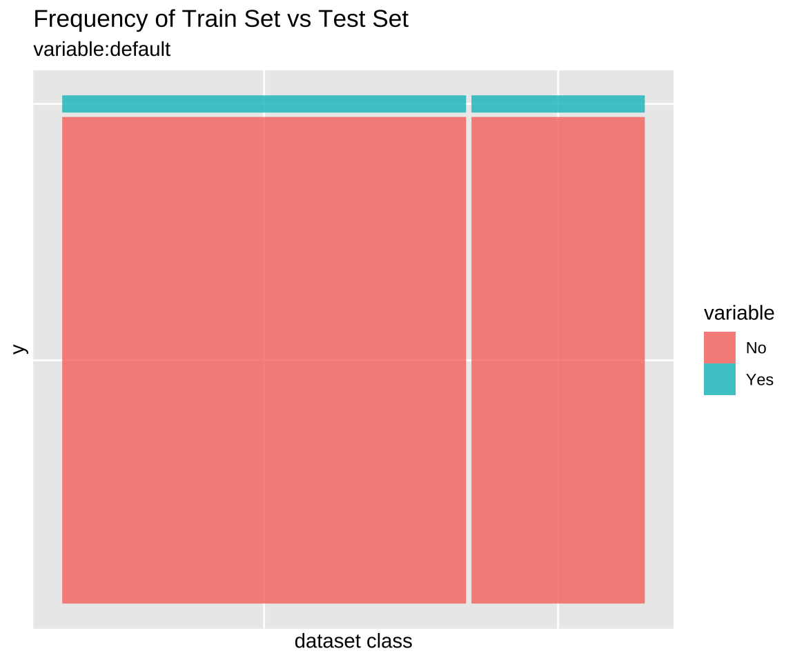
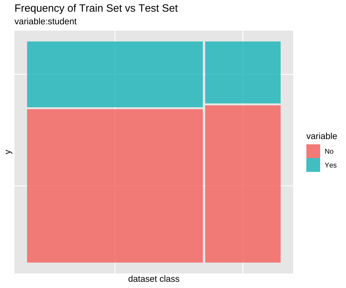
Comparison of categorical variables with compare_target_category()
Compare the statistics of the categorical variables of the train set and test set included in the “split_df” class.
sb %>%
  compare_target_category()
# A tibble: 4 x 5
  variable level train  test abs_diff
  <chr>    <fct> <dbl> <dbl>    <dbl>
1 default  No    96.7  96.7   0.00476
2 default  Yes    3.33  3.33  0.00476
3 student  No    70.0  71.8   1.77
4 student  Yes   30.0  28.2   1.77
# compare variables that are character data types.
sb %>%
  compare_target_category(add_character = TRUE)
# A tibble: 4 x 5
  variable level train  test abs_diff
  <chr>    <fct> <dbl> <dbl>    <dbl>
1 default  No    96.7  96.7   0.00476
2 default  Yes    3.33  3.33  0.00476
3 student  No    70.0  71.8   1.77
4 student  Yes   30.0  28.2   1.77
# display marginal
sb %>%
  compare_target_category(margin = TRUE)
# A tibble: 6 x 5
  variable level    train   test abs_diff
  <chr>    <fct>    <dbl>  <dbl>    <dbl>
1 default  No       96.7   96.7   0.00476
2 default  Yes       3.33   3.33  0.00476
3 default  <Total> 100    100     0.00952
4 student  No       70.0   71.8   1.77
5 student  Yes      30.0   28.2   1.77
6 student  <Total> 100    100     3.54
# student variable only
sb %>%
  compare_target_category(student)
# A tibble: 2 x 5
  variable level train  test abs_diff
  <chr>    <fct> <dbl> <dbl>    <dbl>
1 student  No     70.0  71.8     1.77
2 student  Yes    30.0  28.2     1.77
sb %>%
  compare_target_category(student, margin = TRUE)
# A tibble: 3 x 5
  variable level   train  test abs_diff
  <chr>    <fct>   <dbl> <dbl>    <dbl>
1 student  No       70.0  71.8     1.77
2 student  Yes      30.0  28.2     1.77
3 student  <Total> 100   100       3.54
compare_target_category() returns tbl_df, where the variables have the following.:
- variable : character. categorical variable name
- level : factor. level of categorical variables
- train : numeric. the relative frequency of the level in the train set
- test : numeric. the relative frequency of the level in the test set
- abs_diff : numeric. the absolute value of the difference between two relative frequencies
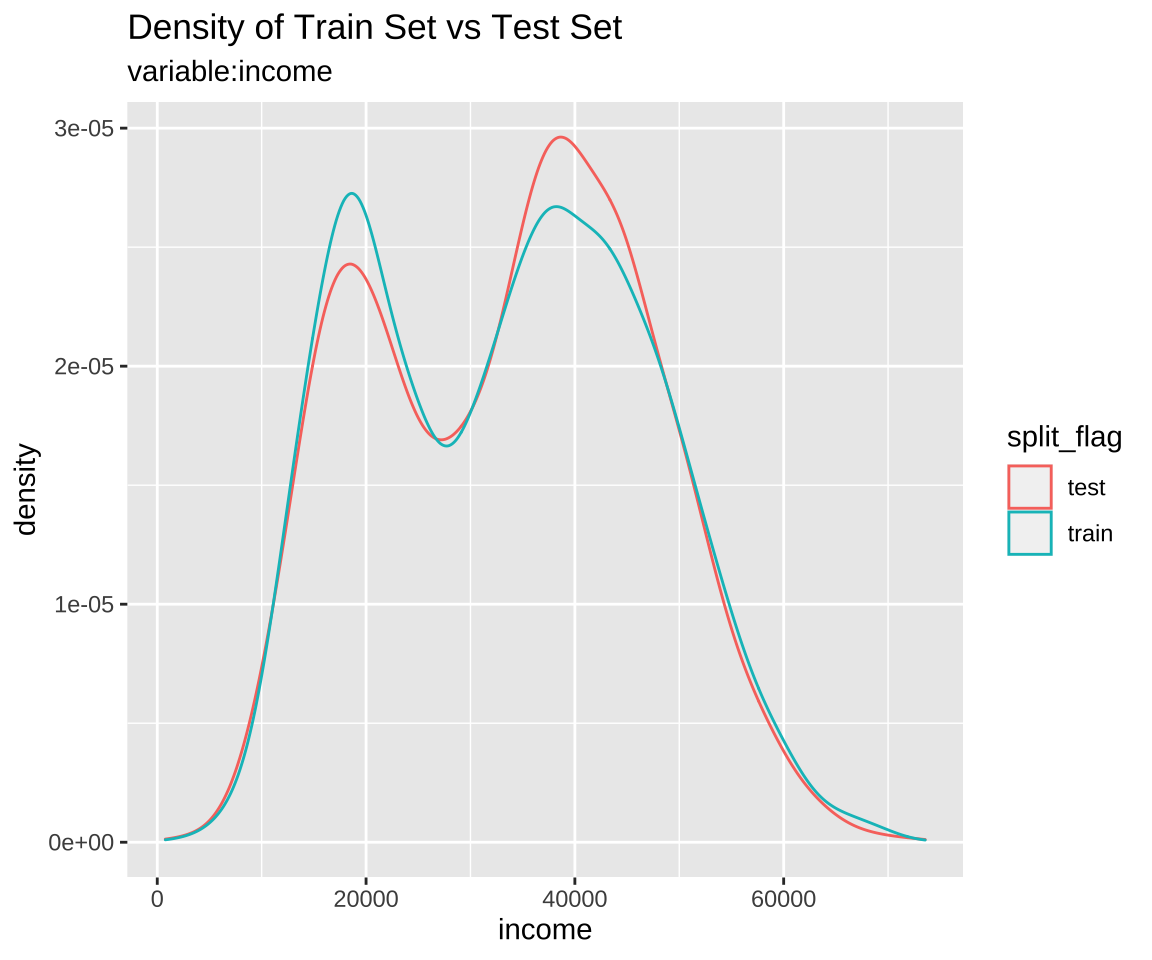
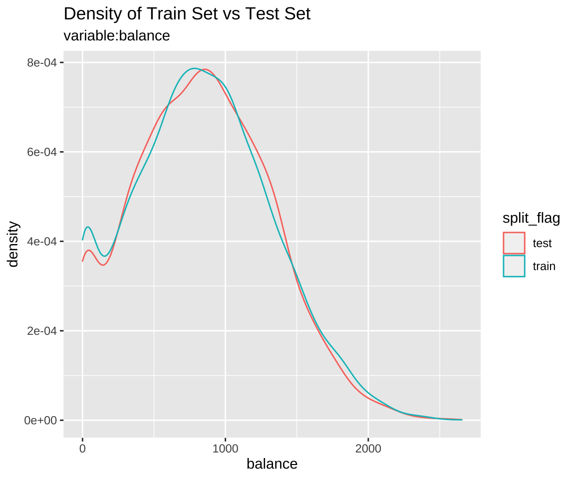
Comparison of numeric variables with compare_target_numeric()
Compare the statistics of the numerical variables of the train set and test set included in the “split_df” class.
sb %>%
  compare_target_numeric()
# A tibble: 2 x 7
  variable train_mean test_mean train_sd test_sd train_z test_z
  <chr>         <dbl>     <dbl>    <dbl>   <dbl>   <dbl>  <dbl>
1 balance        836.      834.     487.    477.    1.72   1.75
2 income       33446.    33684.   13437.  13101.    2.49   2.57
# balance variable only
sb %>%
  compare_target_numeric(balance)
# A tibble: 1 x 7
  variable train_mean test_mean train_sd test_sd train_z test_z
  <chr>         <dbl>     <dbl>    <dbl>   <dbl>   <dbl>  <dbl>
1 balance        836.      834.     487.    477.    1.72   1.75
compare_target_numeric() returns tbl_df, where the variables have the following.:
- variable : character. numeric variable name
- train_mean : numeric. arithmetic mean of train set
- test_mean : numeric. arithmetic mean of test set
- train_sd : numeric. standard deviation of train set
- test_sd : numeric. standard deviation of test set
- train_z : numeric. the arithmetic mean of the train set divided by the standard deviation
- test_z : numeric. the arithmetic mean of the test set divided by the standard deviation
Comparison plot with compare_plot()
Plot compare information of the train set and test set included in the “split_df” class.

Diagnosis of train set and test set with compare_diag()
Diagnosis of similarity between datasets splitted by train set and set included in the “split_df” class.
defaults <- ISLR::Default
defaults$id <- seq(NROW(defaults))

set.seed(1)
defaults[sample(seq(NROW(defaults)), 3), "student"] <- NA
set.seed(2)
defaults[sample(seq(NROW(defaults)), 10), "balance"] <- NA

sb_2 <- defaults %>%
  split_by(default)

sb_2 %>%
  compare_diag()
$missing_value
# A tibble: 2 x 4
  variables train_misscount train_missrate test_missrate
  <chr>               <int>          <dbl>         <dbl>
1 student                 3         0.0429        NA
2 balance                 5         0.0714         0.167

$single_value
# A tibble: 0 x 3
# … with 3 variables: variables <chr>, train_uniq <lgl>,
#   test_uniq <lgl>

$uniq_rate
# A tibble: 0 x 5
# … with 5 variables: variables <chr>, train_uniqcount <int>,
#   train_uniqrate <dbl>, test_uniqcount <int>, test_uniqrate <dbl>

$missing_level
# A tibble: 1 x 4
  variables n_levels train_missing_nlevel test_missing_nlevel
  <chr>        <int>                <int>               <int>
1 student          3                    0                   1
sb_2 %>%
  compare_diag(add_character = TRUE)
$missing_value
# A tibble: 2 x 4
  variables train_misscount train_missrate test_missrate
  <chr>               <int>          <dbl>         <dbl>
1 student                 3         0.0429        NA
2 balance                 5         0.0714         0.167

$single_value
# A tibble: 0 x 3
# … with 3 variables: variables <chr>, train_uniq <lgl>,
#   test_uniq <lgl>

$uniq_rate
# A tibble: 0 x 5
# … with 5 variables: variables <chr>, train_uniqcount <int>,
#   train_uniqrate <dbl>, test_uniqcount <int>, test_uniqrate <dbl>

$missing_level
# A tibble: 1 x 4
  variables n_levels train_missing_nlevel test_missing_nlevel
  <chr>        <int>                <int>               <int>
1 student          3                    0                   1
sb_2 %>%
  compare_diag(uniq_thres = 0.0005)
$missing_value
# A tibble: 2 x 4
  variables train_misscount train_missrate test_missrate
  <chr>               <int>          <dbl>         <dbl>
1 student                 3         0.0429        NA
2 balance                 5         0.0714         0.167

$single_value
# A tibble: 0 x 3
# … with 3 variables: variables <chr>, train_uniq <lgl>,
#   test_uniq <lgl>

$uniq_rate
# A tibble: 2 x 5
  variables train_uniqcount train_uniqrate test_uniqcount
  <chr>               <int>          <dbl>          <int>
1 default                NA             NA              2
2 student                NA             NA              2
# … with 1 more variable: test_uniqrate <dbl>

$missing_level
# A tibble: 1 x 4
  variables n_levels train_missing_nlevel test_missing_nlevel
  <chr>        <int>                <int>               <int>
1 student          3                    0                   1
Extract train/test dataset
If you compare the train set with the test set and find that the two datasets are similar, extract the data from the split_df object.
Extract train set or test set with extract_set()
Extract train set or test set from split_df class object.
train <- sb %>%
  extract_set(set = "train")

test <- sb %>%
  extract_set(set = "test")

dim(train)
[1] 7000 4
dim(test)
[1] 3000 4Extract the data to fit the model with sampling_target()
In a target class, the ratio of the majority class to the minority class is not similar and the ratio of the minority class is very small, which is called the imbalanced class.
If target variable is an imbalanced class, the characteristics of the majority class are actively reflected in the model. This model implies an error in predicting the minority class as the majority class. So we have to make the train dataset a balanced class.
sampling_target() performs sampling on the train set of split_df to resolve the imbalanced class.
# under-sampling with random seed
under <- sb %>%
  sampling_target(seed = 1234L)

under %>%
  count(default)
# A tibble: 2 x 2
  default     n
  <fct>   <int>
1 No        233
2 Yes       233
# under-sampling with random seed, and minority class frequency is 40%
under40 <- sb %>%
  sampling_target(seed = 1234L, perc = 40)

under40 %>%
  count(default)
# A tibble: 2 x 2
  default     n
  <fct>   <int>
1 No        349
2 Yes       233
# over-sampling with random seed
over <- sb %>%
  sampling_target(method = "ubOver", seed = 1234L)

over %>%
  count(default)
# A tibble: 2 x 2
  default     n
  <fct>   <int>
1 No       6767
2 Yes      6767
# over-sampling with random seed, and k = 10
over10 <- sb %>%
  sampling_target(method = "ubOver", seed = 1234L, k = 10)

over10 %>%
  count(default)
# A tibble: 2 x 2
  default     n
  <fct>   <int>
1 No       6767
2 Yes      2330
# SMOTE with random seed
smote <- sb %>%
  sampling_target(method = "ubSMOTE", seed = 1234L)

smote %>%
  count(default)
# A tibble: 2 x 2
  default     n
  <fct>   <int>
1 No        932
2 Yes       699
# SMOTE with random seed, and perc.under = 250
smote250 <- sb %>%
  sampling_target(method = "ubSMOTE", seed = 1234L, perc.under = 250)

smote250 %>%
  count(default)
# A tibble: 2 x 2
  default     n
  <fct>   <int>
1 No       1165
2 Yes       699
The argument that specifies the sampling method in sampling_target () is method. “ubUnder” is under-sampling, and “ubOver” is over-sampling, “ubSMOTE” is SMOTE(Synthetic Minority Over-sampling TEchnique).