The plot_normality() visualize distribution information for normality test of the numerical data.
plot_normality(.data, ...)

# S3 method for class 'data.frame'
plot_normality(
  .data,
  ...,
  left = c("log", "sqrt", "log+1", "log+a", "1/x", "x^2", "x^3", "Box-Cox",
    "Yeo-Johnson"),
  right = c("sqrt", "log", "log+1", "log+a", "1/x", "x^2", "x^3", "Box-Cox",
    "Yeo-Johnson"),
  col = "steelblue",
  typographic = TRUE,
  base_family = NULL
)

# S3 method for class 'grouped_df'
plot_normality(
  .data,
  ...,
  left = c("log", "sqrt", "log+1", "log+a", "1/x", "x^2", "x^3", "Box-Cox",
    "Yeo-Johnson"),
  right = c("sqrt", "log", "log+1", "log+a", "1/x", "x^2", "x^3", "Box-Cox",
    "Yeo-Johnson"),
  col = "steelblue",
  typographic = TRUE,
  base_family = NULL
)
Arguments
- .data
a data.frame or a
tbl_df.- ...
one or more unquoted expressions separated by commas. You can treat variable names like they are positions. Positive values select variables; negative values to drop variables. If the first expression is negative, plot_normality() will automatically start with all variables. These arguments are automatically quoted and evaluated in a context where column names represent column positions. They support unquoting and splicing.
See vignette("EDA") for an introduction to these concepts.
- left
character. Specifies the data transformation method to draw the histogram in the lower left corner. The default is "log".
- right
character. Specifies the data transformation method to draw the histogram in the lower right corner. The default is "sqrt".
- col
a color to be used to fill the bars. The default is "steelblue".
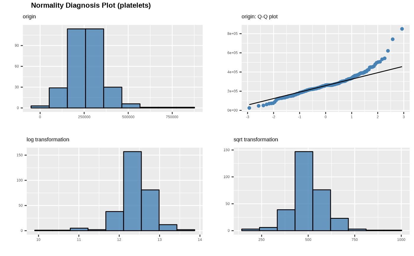
- typographic
logical. Whether to apply focuses on typographic elements to ggplot2 visualization. The default is TRUE. if TRUE provides a base theme that focuses on typographic elements.
- base_family
character. The name of the base font family to use for the visualization. If not specified, the font defined in dlookr is applied. (See details)
Details
The scope of the visualization is the provide a distribution information. Since the plot is drawn for each variable, if you specify more than one variable in the ... argument, the specified number of plots are drawn.
The argument values that left and right can have are as follows.:
"log" : log transformation. log(x)
"log+1" : log transformation. log(x + 1). Used for values that contain 0.
"log+a" : log transformation. log(x + 1 - min(x)). Used for values that contain 0.
"sqrt" : square root transformation.
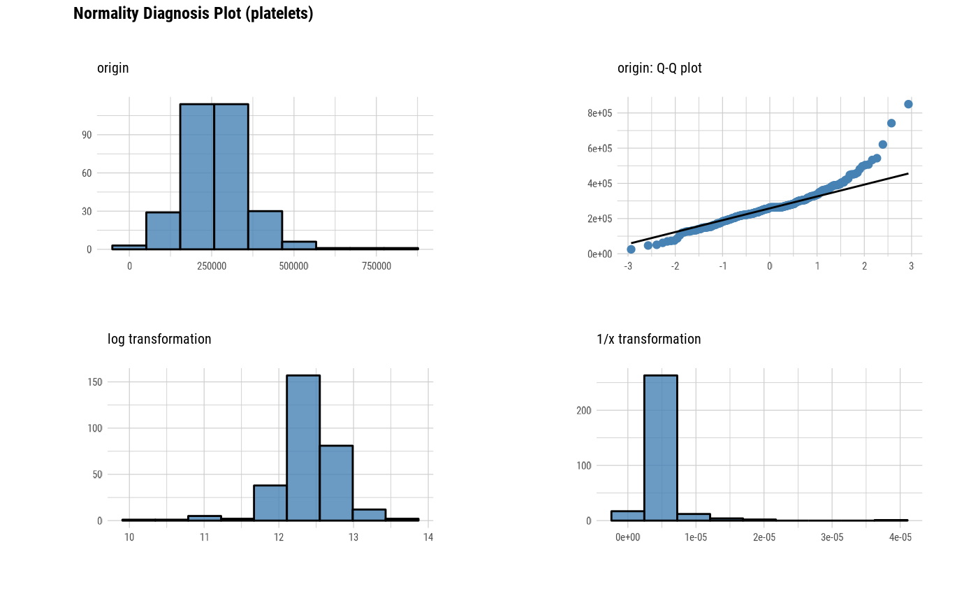
"1/x" : 1 / x transformation
"x^2" : x square transformation
"x^3" : x^3 square transformation
"Box-Cox" : Box-Box transformation
"Yeo-Johnson" : Yeo-Johnson transformation
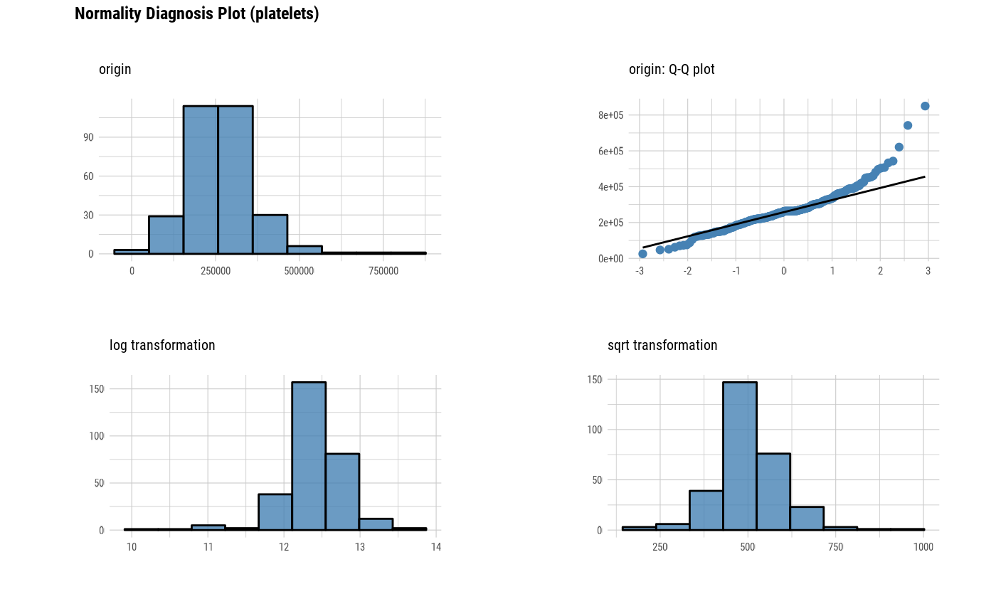
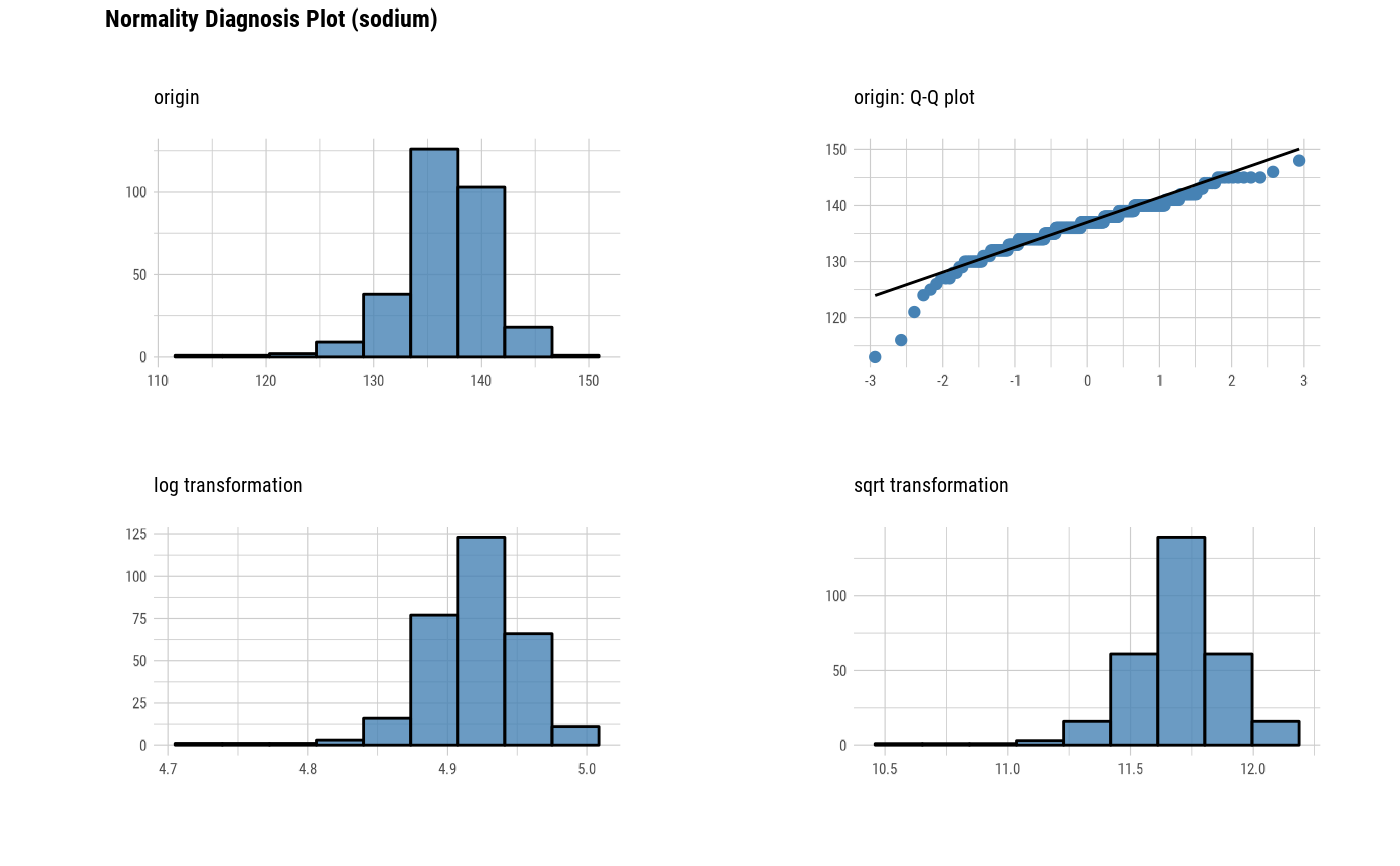
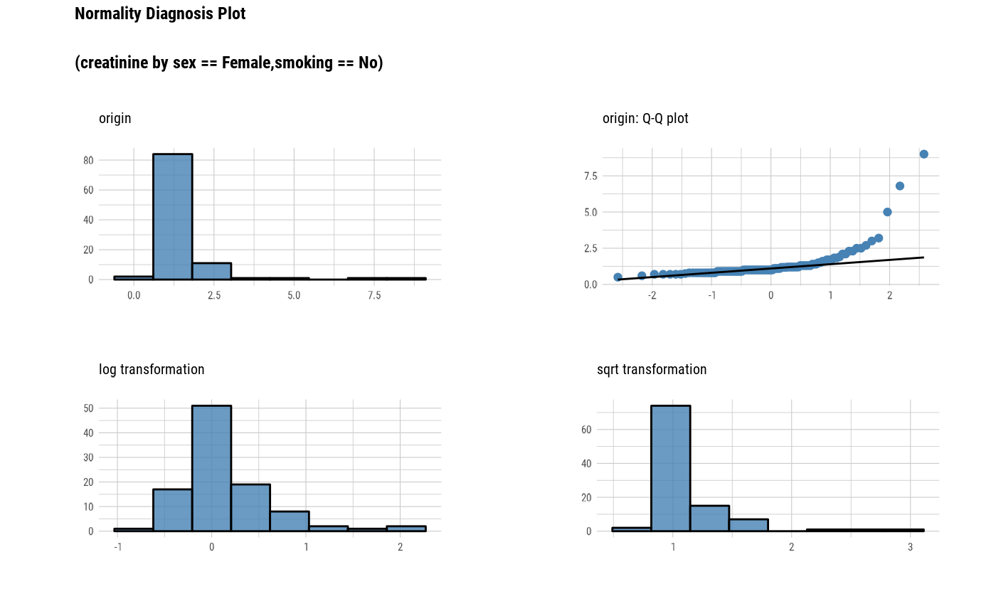
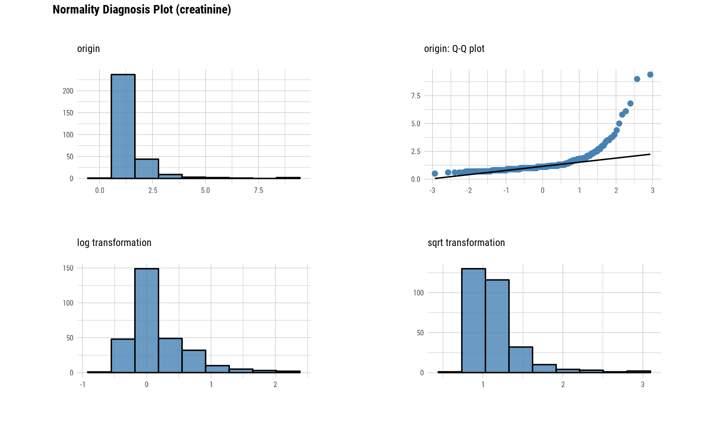
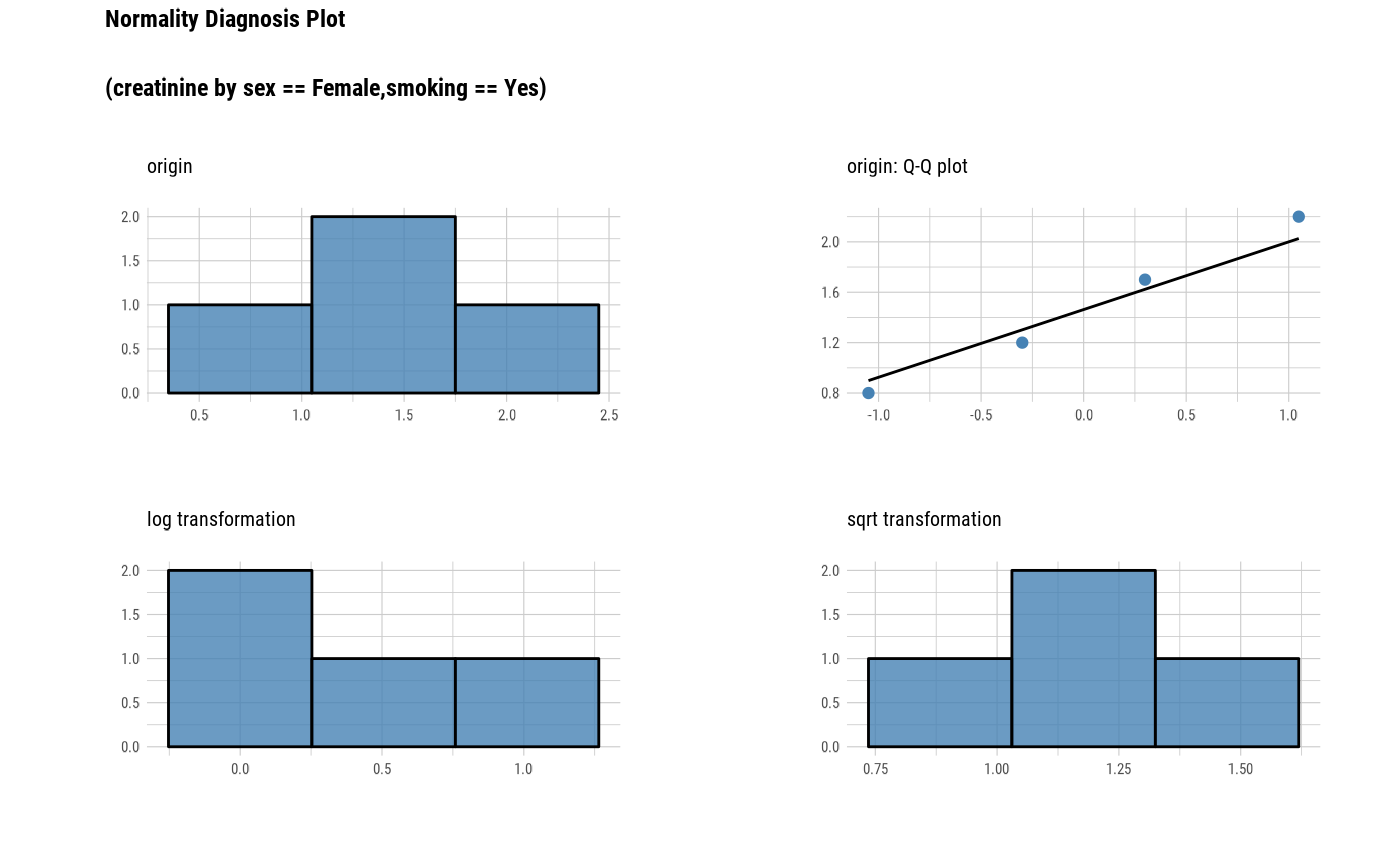
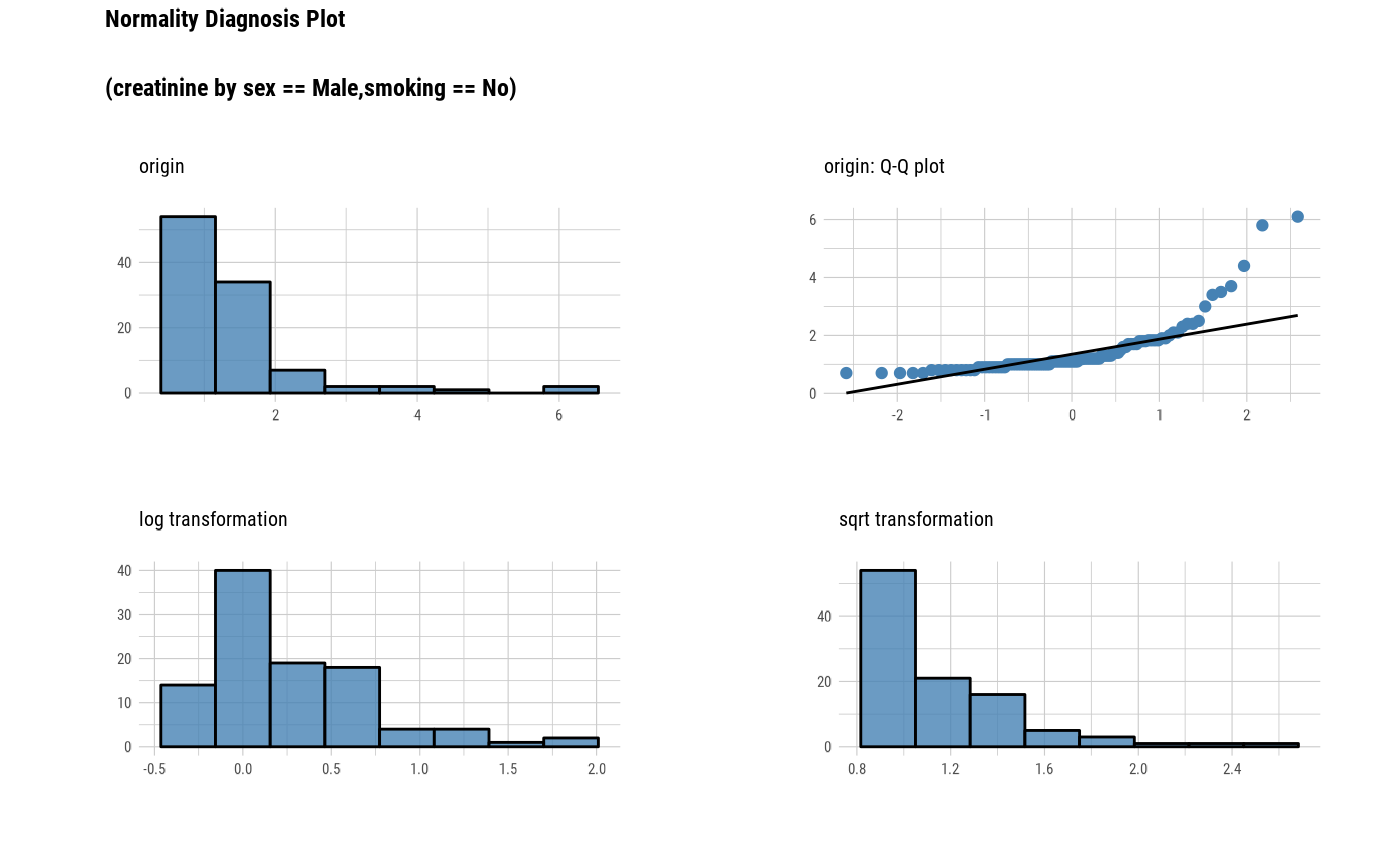
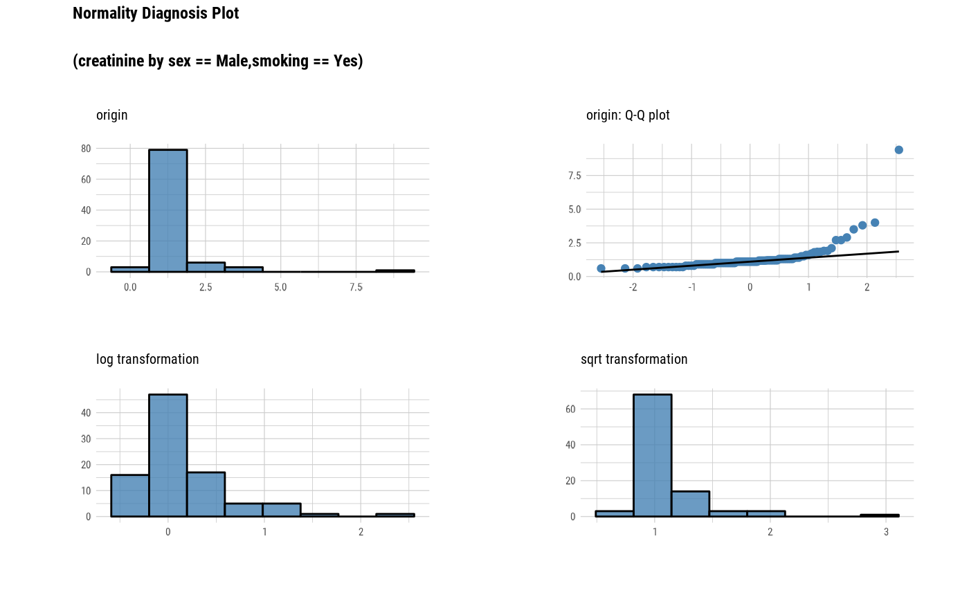
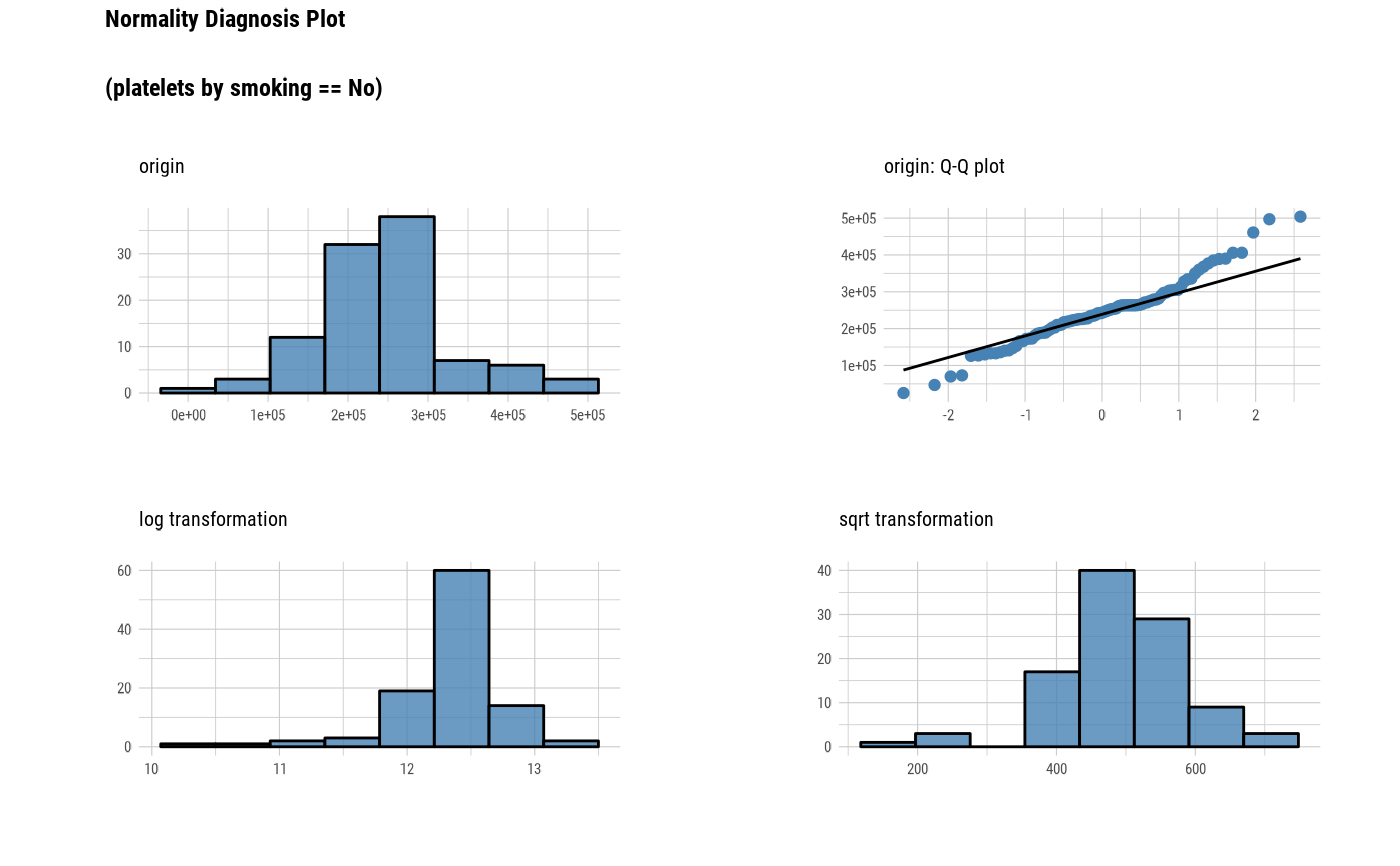
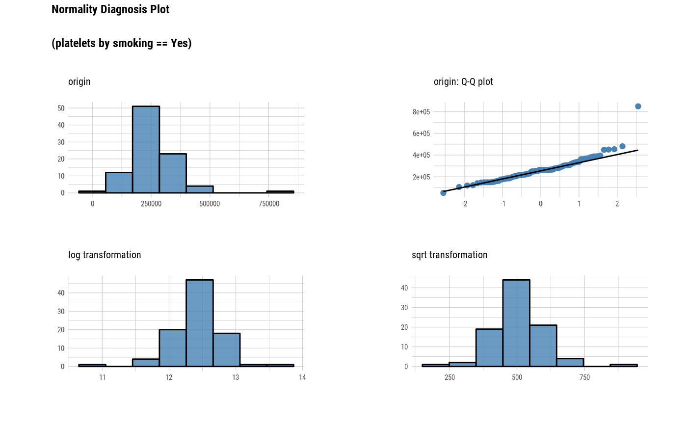
Distribution information
The plot derived from the numerical data visualization is as follows.
histogram by original data
q-q plot by original data
histogram by log transfer data
histogram by square root transfer data
The base_family is selected from "Roboto Condensed", "Liberation Sans Narrow", "NanumSquare", "Noto Sans Korean". If you want to use a different font, use it after loading the Google font with import_google_font().
See also
Examples
# \donttest{
# Visualization of all numerical variables
heartfailure2 <- heartfailure[, c("creatinine", "platelets", "sodium", "sex", "smoking")]
plot_normality(heartfailure2)


 # Select the variable to plot
plot_normality(heartfailure2, platelets, sodium)
# Select the variable to plot
plot_normality(heartfailure2, platelets, sodium)
 # Change the method of transformation
plot_normality(heartfailure2, platelets, right = "1/x")
# Change the method of transformation
plot_normality(heartfailure2, platelets, right = "1/x")
 # Non typographic elements
plot_normality(heartfailure2, platelets, typographic = FALSE)
# Non typographic elements
plot_normality(heartfailure2, platelets, typographic = FALSE)
 # Using dplyr::grouped_df
library(dplyr)
gdata <- group_by(heartfailure2, sex, smoking)
plot_normality(gdata, "creatinine")
# Using dplyr::grouped_df
library(dplyr)
gdata <- group_by(heartfailure2, sex, smoking)
plot_normality(gdata, "creatinine")


 # Using pipes ---------------------------------
# Visualization of all numerical variables
heartfailure2 %>%
plot_normality()
# Using pipes ---------------------------------
# Visualization of all numerical variables
heartfailure2 %>%
plot_normality()

 # Positive values select variables
# heartfailure2 %>%
# plot_normality(platelets, sodium)
# Using pipes & dplyr -------------------------
# Plot 'creatinine' variable by 'sex' and 'smoking'
heartfailure2 %>%
group_by(sex, smoking) %>%
plot_normality(creatinine)
# Positive values select variables
# heartfailure2 %>%
# plot_normality(platelets, sodium)
# Using pipes & dplyr -------------------------
# Plot 'creatinine' variable by 'sex' and 'smoking'
heartfailure2 %>%
group_by(sex, smoking) %>%
plot_normality(creatinine)

 # extract only those with 'sex' variable level is "Male",
# and plot 'platelets' by 'smoking'
heartfailure2 %>%
filter(sex == "Male") %>%
group_by(smoking) %>%
plot_normality(platelets, right = "sqrt")
# extract only those with 'sex' variable level is "Male",
# and plot 'platelets' by 'smoking'
heartfailure2 %>%
filter(sex == "Male") %>%
group_by(smoking) %>%
plot_normality(platelets, right = "sqrt")
 # }
# }