Data quality diagnosis

Preface

After you have acquired the data, you should do the following:

Diagnose data quality.
- If there is a problem with data quality,
- The data must be corrected or re-acquired.
Explore data to understand the data and find scenarios for performing the analysis.
Derive new variables or perform variable transformations.

The dlookr package makes these steps fast and easy:

Performs a data diagnosis or automatically generates a data diagnosis report.
Discover data in various ways and automatically generate EDA(exploratory data analysis) reports.
Impute missing values and outliers, resolve skewed data, and categorize continuous variables into categorical variables. And generates an automated report to support it.

This document introduces Data Quality Diagnosis methods provided by the dlookr package. You will learn how to diagnose the quality of tbl_df data that inherits from data.frame and data.frame with functions provided by dlookr.

dlookr increases synergy with dplyr. Particularly in data exploration and data wrangling, it increases the efficiency of the tidyverse package group.

Supported data structures

Data diagnosis supports the following data structures.

data frame: data.frame class.
data table: tbl_df class.
table of DBMS: table of the DBMS through tbl_dbi.
- Use dplyr as the back-end interface for any DBI-compatible database.

Data: nycflights13

To illustrate the primary use of the dlookr package, use the flights data from the nycflights13 package. The flights data frame is data about departure and arrival on all flights departing from NYC in 2013.

dim(flights)
[1] 3000   19
flights
 [38;5;246m# A tibble: 3,000 × 19 [39m
   year month   day dep_time sched_dep_time dep_delay arr_time sched_arr_time
   [3m [38;5;246m<int> [39m [23m  [3m [38;5;246m<int> [39m [23m  [3m [38;5;246m<int> [39m [23m     [3m [38;5;246m<int> [39m [23m           [3m [38;5;246m<int> [39m [23m      [3m [38;5;246m<dbl> [39m [23m     [3m [38;5;246m<int> [39m [23m           [3m [38;5;246m<int> [39m [23m
 [38;5;250m1 [39m   [4m2 [24m013     6    17      [4m1 [24m033            [4m1 [24m040        - [31m7 [39m      [4m1 [24m246            [4m1 [24m309
 [38;5;250m2 [39m   [4m2 [24m013    12    26      [4m1 [24m343            [4m1 [24m329        14      [4m1 [24m658            [4m1 [24m624
 [38;5;250m3 [39m   [4m2 [24m013     8    26      [4m1 [24m258            [4m1 [24m218        40      [4m1 [24m510            [4m1 [24m516
 [38;5;250m4 [39m   [4m2 [24m013     8    17      [4m1 [24m558            [4m1 [24m600        - [31m2 [39m      [4m1 [24m835            [4m1 [24m849
 [38;5;246m# ℹ 2,996 more rows [39m
 [38;5;246m# ℹ 11 more variables: arr_delay <dbl>, carrier <chr>, flight <int>, [39m
 [38;5;246m#   tailnum <chr>, origin <chr>, dest <chr>, air_time <dbl>, distance <dbl>, [39m
 [38;5;246m#   hour <dbl>, minute <dbl>, time_hour <dttm> [39m

Data diagnosis

dlookr aims to diagnose the data and select variables that can not be used for data analysis or to find the variables that need calibration.:

diagnose() provides basic diagnostic information for variables.
diagnose_category() provides detailed diagnostic information for categorical variables.
diagnose_numeric() provides detailed diagnostic information for numerical variables.
diagnose_outlier() and plot_outlier() provide information and visualization of outliers.

General diagnosis of all variables with `diagnose()`

diagnose() allows the diagnosis of variables in a data frame. Like the function of dplyr, the first argument is the tibble (or data frame). The second and subsequent arguments refer to variables within that data frame.

The variables of the tbl_df object returned by diagnose () are as follows.

variables: variable names
types: the data type of the variables
missing_count: number of missing values
missing_percent: percentage of missing value
unique_count: number of unique value
unique_rate: rate of unique value. unique_count / number of observation

For example, we can diagnose all variables in flights:

diagnose(flights)
 [38;5;246m# A tibble: 19 × 6 [39m
  variables types   missing_count missing_percent unique_count unique_rate
   [3m [38;5;246m<chr> [39m [23m      [3m [38;5;246m<chr> [39m [23m            [3m [38;5;246m<int> [39m [23m            [3m [38;5;246m<dbl> [39m [23m         [3m [38;5;246m<int> [39m [23m        [3m [38;5;246m<dbl> [39m [23m
 [38;5;250m1 [39m year      integer             0            0               1    0.000 [4m3 [24m [4m3 [24m [4m3 [24m
 [38;5;250m2 [39m month     integer             0            0              12    0.004   
 [38;5;250m3 [39m day       integer             0            0              31    0.010 [4m3 [24m  
 [38;5;250m4 [39m dep_time  integer            82            2.73          982    0.327   
 [38;5;246m# ℹ 15 more rows [39m

Missing Value(NA): Variables with many missing values, i.e., those with a missing_percent close to 100, should be excluded from the analysis.
Unique value: If the data type is not numeric (integer, numeric) and the number of unique values equals the number of observations (unique_rate = 1), the variable will likely be an identifier. Therefore, this variable is also not suitable for the analysis mode

year can be considered not to be used in the analysis model since unique_count is 1. However, you do not have to remove it if you configure date as a combination of year, month, and day.

For example, we can diagnose only a few selected variables:

# Select columns by name
diagnose(flights, year, month, day)
 [38;5;246m# A tibble: 3 × 6 [39m
  variables types   missing_count missing_percent unique_count unique_rate
   [3m [38;5;246m<chr> [39m [23m      [3m [38;5;246m<chr> [39m [23m            [3m [38;5;246m<int> [39m [23m            [3m [38;5;246m<dbl> [39m [23m         [3m [38;5;246m<int> [39m [23m        [3m [38;5;246m<dbl> [39m [23m
 [38;5;250m1 [39m year      integer             0               0            1    0.000 [4m3 [24m [4m3 [24m [4m3 [24m
 [38;5;250m2 [39m month     integer             0               0           12    0.004   
 [38;5;250m3 [39m day       integer             0               0           31    0.010 [4m3 [24m  
# Select all columns between year and day (include)
diagnose(flights, year:day)
 [38;5;246m# A tibble: 3 × 6 [39m
  variables types   missing_count missing_percent unique_count unique_rate
   [3m [38;5;246m<chr> [39m [23m      [3m [38;5;246m<chr> [39m [23m            [3m [38;5;246m<int> [39m [23m            [3m [38;5;246m<dbl> [39m [23m         [3m [38;5;246m<int> [39m [23m        [3m [38;5;246m<dbl> [39m [23m
 [38;5;250m1 [39m year      integer             0               0            1    0.000 [4m3 [24m [4m3 [24m [4m3 [24m
 [38;5;250m2 [39m month     integer             0               0           12    0.004   
 [38;5;250m3 [39m day       integer             0               0           31    0.010 [4m3 [24m  
# Select all columns except those from year to day (exclude)
diagnose(flights, -(year:day))
 [38;5;246m# A tibble: 16 × 6 [39m
  variables      types   missing_count missing_percent unique_count unique_rate
   [3m [38;5;246m<chr> [39m [23m           [3m [38;5;246m<chr> [39m [23m            [3m [38;5;246m<int> [39m [23m            [3m [38;5;246m<dbl> [39m [23m         [3m [38;5;246m<int> [39m [23m        [3m [38;5;246m<dbl> [39m [23m
 [38;5;250m1 [39m dep_time       integer            82            2.73          982       0.327
 [38;5;250m2 [39m sched_dep_time integer             0            0             588       0.196
 [38;5;250m3 [39m dep_delay      numeric            82            2.73          204       0.068
 [38;5;250m4 [39m arr_time       integer            87            2.9           [4m1 [24m010       0.337
 [38;5;246m# ℹ 12 more rows [39m

Using dplyr, variables, including missing values, can be sorted by the weight of missing values.:

flights %>%
  diagnose() %>%
  select(-unique_count, -unique_rate) %>% 
  filter(missing_count > 0) %>% 
  arrange(desc(missing_count))
 [38;5;246m# A tibble: 6 × 4 [39m
  variables types   missing_count missing_percent
   [3m [38;5;246m<chr> [39m [23m      [3m [38;5;246m<chr> [39m [23m            [3m [38;5;246m<int> [39m [23m            [3m [38;5;246m<dbl> [39m [23m
 [38;5;250m1 [39m arr_delay numeric            89            2.97
 [38;5;250m2 [39m air_time  numeric            89            2.97
 [38;5;250m3 [39m arr_time  integer            87            2.9 
 [38;5;250m4 [39m dep_time  integer            82            2.73
 [38;5;246m# ℹ 2 more rows [39m

Diagnosis of numeric variables with `diagnose_numeric()`

diagnose_numeric() diagnoses numeric(continuous and discrete) variables in a data frame. Usage is the same as diagnose() but returns more diagnostic information. However, if you specify a non-numeric variable in the second and subsequent argument list, the variable is automatically ignored.

The variables of the tbl_df object returned by diagnose_numeric() are as follows.

min: minimum value
Q1: 1/4 quartile, 25th percentile
mean: arithmetic mean
median: median, 50th percentile
Q3: 3/4 quartile, 75th percentile
max: maximum value
zero: number of observations with a value of 0
minus: number of observations with negative numbers
outlier: number of outliers

The summary() function summarizes the distribution of individual variables in the data frame and outputs it to the console. The summary values of numeric variables are min, Q1, mean, median, Q3 and max, which help to understand the data distribution.

However, the result displayed on the console has the disadvantage that the analyst has to look at it with the eyes. However, when the summary information is returned in a data frame structure such as tbl_df, the scope of utilization is expanded. diagnose_numeric() supports this.

zero, minus, and outlier are helpful measures to diagnose data integrity. For example, in some cases, numerical data cannot have zero or negative numbers. A numeric variable, employee salary, cannot have negative numbers or zeros. Therefore, this variable should be checked for the inclusion of zero or negative numbers in the data diagnosis process.

diagnose_numeric() can diagnose all numeric variables of flights as follows.:

diagnose_numeric(flights)
 [38;5;246m# A tibble: 14 × 10 [39m
  variables   min    Q1    mean median      Q3   max  zero minus outlier
   [3m [38;5;246m<chr> [39m [23m      [3m [38;5;246m<dbl> [39m [23m  [3m [38;5;246m<dbl> [39m [23m    [3m [38;5;246m<dbl> [39m [23m   [3m [38;5;246m<dbl> [39m [23m    [3m [38;5;246m<dbl> [39m [23m  [3m [38;5;246m<dbl> [39m [23m  [3m [38;5;246m<int> [39m [23m  [3m [38;5;246m<int> [39m [23m    [3m [38;5;246m<int> [39m [23m
 [38;5;250m1 [39m year        [4m2 [24m013  [4m2 [24m013   [4m2 [24m013       [4m2 [24m013  [4m2 [24m013      [4m2 [24m013     0     0       0
 [38;5;250m2 [39m month         1    4     6.54      7    9.25    12     0     0       0
 [38;5;250m3 [39m day           1    8    15.8      16   23       31     0     0       0
 [38;5;250m4 [39m dep_time      1  905.  [4m1 [24m354.      [4m1 [24m417  [4m1 [24m755      [4m2 [24m359     0     0       0
 [38;5;246m# ℹ 10 more rows [39m

If a numeric variable can not logically have a negative or zero value, it can be used with filter() to easily find a variable that does not logically match:

diagnose_numeric(flights) %>% 
  filter(minus > 0 | zero > 0) 
 [38;5;246m# A tibble: 3 × 10 [39m
  variables   min     Q1  mean median    Q3   max  zero minus outlier
   [3m [38;5;246m<chr> [39m [23m      [3m [38;5;246m<dbl> [39m [23m   [3m [38;5;246m<dbl> [39m [23m  [3m [38;5;246m<dbl> [39m [23m   [3m [38;5;246m<dbl> [39m [23m  [3m [38;5;246m<dbl> [39m [23m  [3m [38;5;246m<dbl> [39m [23m  [3m [38;5;246m<int> [39m [23m  [3m [38;5;246m<int> [39m [23m    [3m [38;5;246m<int> [39m [23m
 [38;5;250m1 [39m dep_delay   - [31m22 [39m  - [31m5 [39m    13.6      - [31m1 [39m    12   [4m1 [24m126   143   [4m1 [24m618     401
 [38;5;250m2 [39m arr_delay   - [31m70 [39m - [31m17 [39m     7.13     - [31m5 [39m    15   [4m1 [24m109    43   [4m1 [24m686     250
 [38;5;250m3 [39m minute        0   9.75 26.4      29    44    59   527     0       0

Diagnosis of categorical variables with `diagnose_category()`

diagnose_category() diagnoses the categorical(factor, ordered, character) variables of a data frame. The usage is similar to diagnose() but returns more diagnostic information. The variable is automatically ignored if you specify a non-categorical variable in the second and subsequent argument list.

The top argument specifies the number of levels to return for each variable. The default is 10, which returns the top 10 levels. Of course, if the number of levels is less than 10, all levels are returned.

The variables of the tbl_df object returned by diagnose_category() are as follows.

variables: variable names
levels: level names
N: number of observation
freq: number of observation at the levels
ratio: percentage of observation at the levels
rank: rank of occupancy ratio of levels

`diagnose_category() can diagnose all categorical variables of flights as follows.:

diagnose_category(flights)
 [38;5;246m# A tibble: 43 × 6 [39m
  variables levels     N  freq ratio  rank
   [3m [38;5;246m<chr> [39m [23m      [3m [38;5;246m<chr> [39m [23m   [3m [38;5;246m<int> [39m [23m  [3m [38;5;246m<int> [39m [23m  [3m [38;5;246m<dbl> [39m [23m  [3m [38;5;246m<int> [39m [23m
 [38;5;250m1 [39m carrier   UA       [4m3 [24m000   551  18.4     1
 [38;5;250m2 [39m carrier   EV       [4m3 [24m000   493  16.4     2
 [38;5;250m3 [39m carrier   B6       [4m3 [24m000   490  16.3     3
 [38;5;250m4 [39m carrier   DL       [4m3 [24m000   423  14.1     4
 [38;5;246m# ℹ 39 more rows [39m

In collaboration with filter() in the dplyr package, we can see that the tailnum variable is ranked in top 1 with 2,512 missing values in the case where the missing value is included in the top 10:

diagnose_category(flights) %>% 
  filter(is.na(levels))
 [38;5;246m# A tibble: 1 × 6 [39m
  variables levels     N  freq ratio  rank
   [3m [38;5;246m<chr> [39m [23m      [3m [38;5;246m<chr> [39m [23m   [3m [38;5;246m<int> [39m [23m  [3m [38;5;246m<int> [39m [23m  [3m [38;5;246m<dbl> [39m [23m  [3m [38;5;246m<int> [39m [23m
 [38;5;250m1 [39m tailnum    [31mNA [39m       [4m3 [24m000    23 0.767     1

The following example returns a list where the level’s relative percentage is 0.01% or less. Note that the value of the top argument is set to a large value, such as 500. If the default value of 10 were used, values below 0.01% would not be included in the list:

flights %>%
  diagnose_category(top = 500)  %>%
  filter(ratio <= 0.01)
 [38;5;246m# A tibble: 0 × 6 [39m
 [38;5;246m# ℹ 6 variables: variables <chr>, levels <chr>, N <int>, freq <int>, [39m
 [38;5;246m#   ratio <dbl>, rank <int> [39m

In the analytics model, you can also consider removing levels where the relative frequency is minimal in the observations or, if possible, combining them together.

Diagnosing outliers with `diagnose_outlier()`

diagnose_outlier() diagnoses the outliers of the data frame’s numeric (continuous and discrete) variables. The usage is the same as diagnose().

The variables of the tbl_df object returned by diagnose_outlier() are as follows.

outliers_cnt: number of outliers
outliers_ratio: percent of outliers
outliers_mean: arithmetic average of outliers
with_mean: arithmetic average of with outliers
without_mean: arithmetic average of without outliers

diagnose_outlier() can diagnose outliers of all numerical variables on flights as follows:

diagnose_outlier(flights)
 [38;5;246m# A tibble: 14 × 6 [39m
  variables outliers_cnt outliers_ratio outliers_mean with_mean without_mean
   [3m [38;5;246m<chr> [39m [23m             [3m [38;5;246m<int> [39m [23m           [3m [38;5;246m<dbl> [39m [23m          [3m [38;5;246m<dbl> [39m [23m      [3m [38;5;246m<dbl> [39m [23m         [3m [38;5;246m<dbl> [39m [23m
 [38;5;250m1 [39m year                 0              0            [31mNaN [39m    [4m2 [24m013          [4m2 [24m013   
 [38;5;250m2 [39m month                0              0            [31mNaN [39m      6.54         6.54
 [38;5;250m3 [39m day                  0              0            [31mNaN [39m     15.8         15.8 
 [38;5;250m4 [39m dep_time             0              0            [31mNaN [39m    [4m1 [24m354.         [4m1 [24m354.  
 [38;5;246m# ℹ 10 more rows [39m

Numeric variables that contained outliers are easily found with filter().:

diagnose_outlier(flights) %>% 
  filter(outliers_cnt > 0) 
 [38;5;246m# A tibble: 4 × 6 [39m
  variables outliers_cnt outliers_ratio outliers_mean with_mean without_mean
   [3m [38;5;246m<chr> [39m [23m             [3m [38;5;246m<int> [39m [23m           [3m [38;5;246m<dbl> [39m [23m          [3m [38;5;246m<dbl> [39m [23m      [3m [38;5;246m<dbl> [39m [23m         [3m [38;5;246m<dbl> [39m [23m
 [38;5;250m1 [39m dep_delay          401          13.4           94.4     13.6         0.722
 [38;5;250m2 [39m arr_delay          250           8.33         121.       7.13       - [31m3 [39m [31m. [39m [31m52 [39m 
 [38;5;250m3 [39m air_time            38           1.27         389.     149.        146.   
 [38;5;250m4 [39m distance             3           0.1          [4m4 [24m970.     [4m1 [24m029.        [4m1 [24m025.

The following example finds a numeric variable with an outlier ratio of 5% or more and then returns the result of dividing the mean of outliers by the overall mean in descending order:

diagnose_outlier(flights) %>% 
  filter(outliers_ratio > 5) %>% 
  mutate(rate = outliers_mean / with_mean) %>% 
  arrange(desc(rate)) %>% 
  select(-outliers_cnt)
 [38;5;246m# A tibble: 2 × 6 [39m
  variables outliers_ratio outliers_mean with_mean without_mean  rate
   [3m [38;5;246m<chr> [39m [23m               [3m [38;5;246m<dbl> [39m [23m          [3m [38;5;246m<dbl> [39m [23m      [3m [38;5;246m<dbl> [39m [23m         [3m [38;5;246m<dbl> [39m [23m  [3m [38;5;246m<dbl> [39m [23m
 [38;5;250m1 [39m arr_delay           8.33         121.       7.13       - [31m3 [39m [31m. [39m [31m52 [39m  16.9 
 [38;5;250m2 [39m dep_delay          13.4           94.4     13.6         0.722  6.94

In cases where the mean of the outliers is large relative to the overall average, it may be desirable to impute or remove the outliers.

Visualization of outliers using `plot_outlier()`

plot_outlier() visualizes outliers of numerical variables(continuous and discrete) of data.frame. Usage is the same as diagnose().

The plot derived from the numerical data diagnosis is as follows.

With outliers box plot
Without outliers box plot
With outliers histogram
Without outliers histogram

plot_outlier() can visualize an outliers in the arr_delay variable of flights as follows:

flights %>%
  plot_outlier(arr_delay)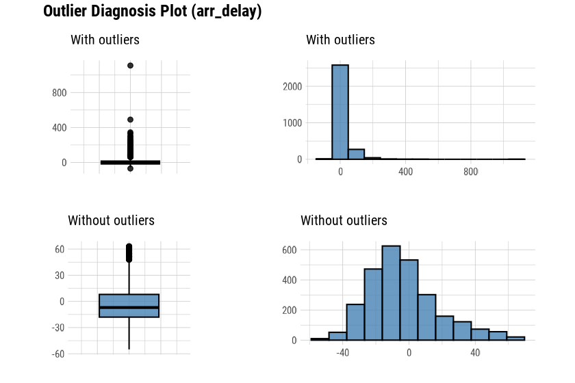

The following example uses diagnose_outlier(), plot_outlier(), and dplyr packages to visualize all numerical variables with an outlier ratio of 5% or higher.

flights %>%
  plot_outlier(diagnose_outlier(flights) %>% 
                 filter(outliers_ratio >= 5) %>% 
                 select(variables) %>% 
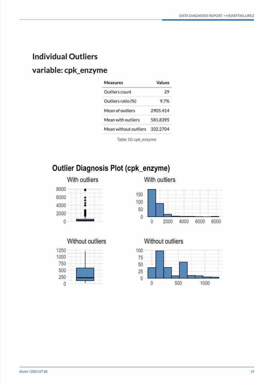
                 unlist())

Analysts should look at the visualization results to decide whether to remove or replace outliers. Sometimes, you should consider removing variables with outliers from the data analysis model.

Looking at the visualization results, arr_delay shows that the observed values without outliers are similar to the normal distribution. In the case of a linear model, we might consider removing or imputing outliers.

Visualization for missing values

It is essential to look at the missing values of individual variables, but it is also important to look at the relationship between the variables, including the missing values.

dlookr provides a visualization tool that looks at the relationship of variables, including missing values.

visualize pareto chart using `plot_na_pareto()`

plot_na_pareto() draws a Pareto chart by collecting variables, including missing values.

mice::boys %>% 
  plot_na_pareto(col = "blue")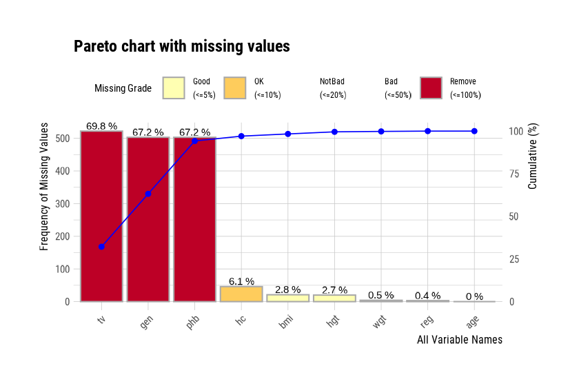

The default value of the only_na argument is FALSE, which includes variables that do not contain missing values. Still, only variables containing missing values are visualized if this value is set to TRUE. The variable age was excluded from this plot.

mice::boys %>% 
  plot_na_pareto(only_na = TRUE, main = "Pareto Chart for mice::boys")

The rating of the variable is expressed as a proportion of missing values. It is calculated as the ratio of missing values. If it is [0, 0.05), it is Good, if it is [0.05, 0.4) it is OK, if it is [0.4, 0.8) it is Bad, and if it is [0.8, 1.0] it is Remove. You can override this grade using the grade argument as follows:

mice::boys %>% 
  plot_na_pareto(grade = list(High = 0.1, Middle = 0.6, Low = 1), relative = TRUE)

If the plot argument is set to FALSE, information about missing values is returned instead of plotting.

plot_na_pareto(mice::boys, only_na = TRUE, plot = FALSE)

visualize combination chart using `plot_na_hclust()`

It is essential to look at the relationship between variables, including missing values. plot_na_hclust() visualizes the relationship of variables that contain missing values. This function rearranges the positions of variables using hierarchical clustering. Then, the expression of the missing value is visualized by grouping similar variables.

mice::boys %>% 
  plot_na_hclust(main = "Distribution of missing value")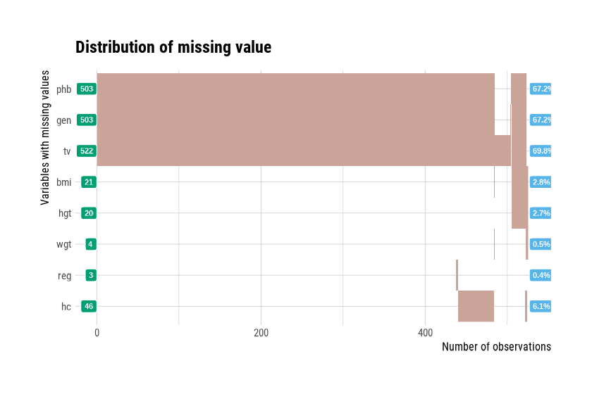

visualize combination chart using `plot_na_intersect()`

plot_na_intersect() visualizes the combinations of missing values across cases.

The visualization consists of four parts. The bottom left, which is the most basic, visualizes the case of cross(intersection)-combination. The x-axis is the variable including the missing value, and the y-axis represents the case of a combination of variables. And on the marginal of the two axes, the frequency of the case is expressed as a bar graph. Finally, the visualization at the top right expresses the number of variables, including missing values in the data set, and the number of observations, including missing values and complete cases.

This example visualizes the combination of variables that include missing values.

mice::boys %>% 
  plot_na_intersect()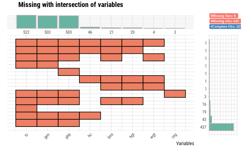

If the n_vars argument is used, only the top n variables containing many missing values are visualized.

mice::boys %>%
  plot_na_intersect(n_vars = 5)

If you use the n_intersacts argument, only the top n numbers of variable combinations(intersection), including missing values, are visualized. Suppose you want to visualize the combination variables, that includes missing values and complete cases. You just add only_na = FALSE.

mice::boys %>%
  plot_na_intersect(only_na = FALSE, n_intersacts = 7)

Automated report

dlookr provides two automated data diagnostic reports:

Web page-based dynamic reports can perform in-depth analysis through visualization and statistical tables.
Static reports generated as pdf files or html files can be archived as output of data analysis.

Create a diagnostic report using `diagnose_web_report()`

diagnose_web_report() creates a dynamic report for objects inherited from data.frame(tbl_df, tbl, etc) or data.frame.

Contents of dynamic web report

The contents of the report are as follows.:

Overview
- Data Structures
  - Data Structures
  - Data Types
  - Job Informations
- Warnings
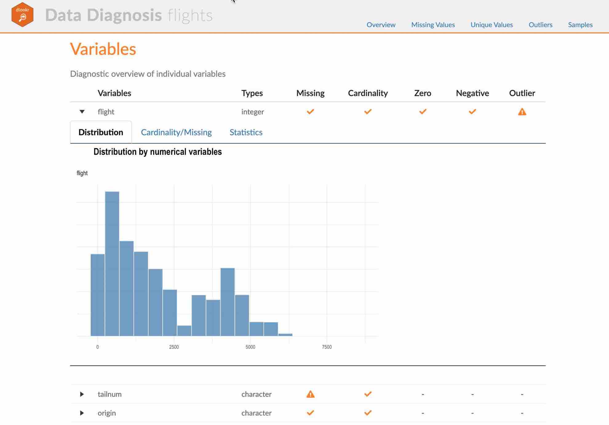
- Variables
Missing Values
- List of Missing Values
- Visualization
Unique Values
- Categorical Variables
- Numerical Variables
Outliers
Samples
- Duplicated
- Heads
- Tails

Some arguments for dynamic web report

diagnose_web_report() generates various reports with the following arguments.

output_file
- name of the generated file.
output_dir
- name of the directory to generate report file.
title
- title of the report.
subtitle
- subtitle of the report.
author
- author of the report.
title_color
- color of title.
thres_uniq_cat
- threshold to use for “Unique Values - Categorical Variables”.
thres_uniq_num
- threshold to use for “Unique Values - Numerical Variables”.
logo_img
- name of the logo image file on the top left.
create_date
- The date on which the report is generated.
theme
- name of theme for report. Support “orange” and “blue”.
sample_percent
- Sample percent of data for performing Diagnosis.

The following script creates a quality diagnosis report for the tbl_df class object, flights.

flights %>%
  diagnose_web_report(subtitle = "flights", output_dir = "./", 
                      output_file = "Diagn.html", theme = "blue")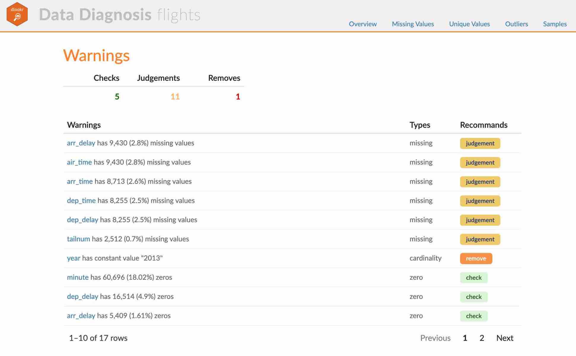

Screenshot of dynamic report

The part of the report is shown in the following figure.:

The part of the report

The dynamic contents of the report are shown in the following figure.:

The dynamic contents of the report

Create a diagnostic report using `diagnose_paged_report()`

diagnose_paged_report() create static report for object inherited from data.frame(tbl_df, tbl, etc) or data.frame.

Contents of static paged report

The contents of the report are as follows.:

Overview
- Data Structures
- Job Informations
- Warnings
- Variables
Missing Values
- List of Missing Values
- Visualization
Unique Values
- Categorical Variables
- Numerical Variables
Categorical Variable Diagnosis
- Top Ranks
Numerical Variable Diagnosis
- Distribution
  - Zero Values
  - Minus Values
- Outliers
  - List of Outliers
  - Individual Outliers

Some arguments for static paged report

diagnose_paged_report() generates various reports with the following arguments.

output_format
- report output type. Choose either “pdf” or “html”.
output_file
- name of the generated file.
output_dir
- name of the directory to generate report file.
title
- title of the report.
subtitle
- subtitle of the report.
abstract_title
- abstract of the report
author
- author of the report.
title_color
- color of title.
subtitle_color
- color of subtitle.
thres_uniq_cat
- threshold to use for “Unique Values - Categorical Variables”.
thres_uniq_num
- threshold to use for “Unique Values - Numerical Variables”.
flag_content_zero
- whether to output “Zero Values” information.
flag_content_minus
- whether to output “Minus Values” information.
flag_content_missing
- whether to output “Missing Value” information.
logo_img
- name of the logo image file on the top left.
cover_img
- name of cover image file on center.
create_date
- The date on which the report is generated.
theme
- name of the theme for the report. Support “orange” and “blue”.
sample_percent
- Sample percent of data for performing Diagnosis.

The following script creates a quality diagnosis report for the tbl_df class object, flights.

flights %>%
  diagnose_paged_report(subtitle = "flights", output_dir = "./",
                        output_file = "Diagn.pdf", theme = "blue")

Screenshot of static report

The cover of the report is shown in the following figure.:

The part of the report

The contents of the report are shown in the following figure.:

The dynamic contents of the report

Diagnosing tables in DBMS

The DBMS table diagnostic function supports In-database mode that performs SQL operations on the DBMS side. If the data size is large, using In-database mode is faster.

It isn’t easy to obtain anomalies or to implement the sampling-based algorithm in SQL of DBMS. So, some functions do not yet support In-database mode. In this case, it is performed in In-memory mode in which table data is brought to the R side and calculated. In this case, if the data size is large, the execution speed may be slow. It supports the collect_size argument, allowing you to import the specified number of data samples into R.

In-database support functions
- diagonse()
- diagnose_category()
In-database not support functions
- diagnose_numeric()
- diagnose_outlier()
- plot_outlier()
- diagnose_web_report()
- diagnose_paged_report()

Preparing table data

Copy the carseats data frame to the SQLite DBMS and create it as a table named TB_CARSEATS. Mysql/MariaDB, PostgreSQL, Oracle DBMS, and other DBMS are also available for your environment.

library(dplyr)

carseats <- Carseats
carseats[sample(seq(NROW(carseats)), 20), "Income"] <- NA
carseats[sample(seq(NROW(carseats)), 5), "Urban"] <- NA

# connect DBMS
con_sqlite <- DBI::dbConnect(RSQLite::SQLite(), ":memory:")

# copy carseats to the DBMS with a table named TB_CARSEATS
copy_to(con_sqlite, carseats, name = "TB_CARSEATS", overwrite = TRUE)

Diagnose data quality of variables in the DBMS

Use dplyr::tbl() to create a tbl_dbi object, then use it as a data frame object. The data argument of all diagnose functions is specified as a tbl_dbi object instead of a data frame object.

# Diagnosis of all columns
con_sqlite %>% 
  tbl("TB_CARSEATS") %>% 
  diagnose()

# Positions values select columns, and In-memory mode
con_sqlite %>% 
  tbl("TB_CARSEATS") %>% 
  diagnose(1, 3, 8, in_database = FALSE)
  
# Positions values select columns, and In-memory mode and collect size is 200
con_sqlite %>% 
  tbl("TB_CARSEATS") %>% 
  diagnose(-8, -9, -10, in_database = FALSE, collect_size = 200)

Diagnose data quality of categorical variables in the DBMS

# Positions values select variables, and In-memory mode and collect size is 200
con_sqlite %>% 
  tbl("TB_CARSEATS") %>% 
  diagnose_category(7, in_database = FALSE, collect_size = 200) 
  
# Positions values select variables
con_sqlite %>% 
  tbl("TB_CARSEATS") %>% 
  diagnose_category(-7)

Diagnose data quality of numerical variables in the DBMS

# Diagnosis of all numerical variables
con_sqlite %>% 
  tbl("TB_CARSEATS") %>% 
  diagnose_numeric()
  
# Positive values select variables, and In-memory mode and collect size is 200
con_sqlite %>% 
  tbl("TB_CARSEATS") %>% 
  diagnose_numeric(Sales, Income, collect_size = 200)

Diagnose outlier of numerical variables in the DBMS

con_sqlite %>% 
  tbl("TB_CARSEATS") %>% 
  diagnose_outlier()  %>%
  filter(outliers_ratio > 1)

Plot outlier information of numerical data diagnosis in the DBMS

# Visualization of numerical variables with a ratio of
# outliers greater than 1%
# the result is same as a data.frame, but not display here. reference above in document.
con_sqlite %>% 
  tbl("TB_CARSEATS") %>% 
  plot_outlier(con_sqlite %>% 
                 tbl("TB_CARSEATS") %>% 
                 diagnose_outlier() %>%
                 filter(outliers_ratio > 1) %>%
                 select(variables) %>%
                 pull())

Reporting the information of data diagnosis for table of thr DBMS

The following shows several examples of creating a data diagnosis report for a DBMS table.

Using the collect_size argument, you can perform data diagnosis with the corresponding number of sample data. If the number of data is huge, use collect_size.

# create web report file. 
con_sqlite %>% 
  tbl("TB_CARSEATS") %>% 
  diagnose_web_report()
  
# create pdf file. file name is Diagn.pdf, and collect size is 350
con_sqlite %>% 
  tbl("TB_CARSEATS") %>% 
  diagnose_paged_report(collect_size = 350, output_file = "Diagn.pdf")

Choonghyun Ryu

2024-02-15

Preface

Supported data structures

Data: nycflights13

Data diagnosis

General diagnosis of all variables with `diagnose()`

Diagnosis of numeric variables with `diagnose_numeric()`

Diagnosis of categorical variables with `diagnose_category()`

Diagnosing outliers with `diagnose_outlier()`

Visualization of outliers using `plot_outlier()`

Visualization for missing values

visualize pareto chart using `plot_na_pareto()`

visualize combination chart using `plot_na_hclust()`

visualize combination chart using `plot_na_intersect()`

Automated report

Create a diagnostic report using `diagnose_web_report()`

Contents of dynamic web report

Some arguments for dynamic web report

Screenshot of dynamic report

Create a diagnostic report using `diagnose_paged_report()`

Contents of static paged report

Some arguments for static paged report

Screenshot of static report

Diagnosing tables in DBMS

Preparing table data

Diagnose data quality of variables in the DBMS

Diagnose data quality of categorical variables in the DBMS

Diagnose data quality of numerical variables in the DBMS

Diagnose outlier of numerical variables in the DBMS

Plot outlier information of numerical data diagnosis in the DBMS

Reporting the information of data diagnosis for table of thr DBMS

Data quality diagnosis

Choonghyun Ryu

2024-02-15

Preface

Supported data structures

Data: nycflights13

Data diagnosis

General diagnosis of all variables with diagnose()

Diagnosis of numeric variables with diagnose_numeric()

Diagnosis of categorical variables with diagnose_category()

Diagnosing outliers with diagnose_outlier()

Visualization of outliers using plot_outlier()

Visualization for missing values

visualize pareto chart using plot_na_pareto()

visualize combination chart using plot_na_hclust()

visualize combination chart using plot_na_intersect()

Automated report

Create a diagnostic report using diagnose_web_report()

Contents of dynamic web report

Some arguments for dynamic web report

Screenshot of dynamic report

Create a diagnostic report using diagnose_paged_report()

Contents of static paged report

Some arguments for static paged report

Screenshot of static report

Diagnosing tables in DBMS

Preparing table data

Diagnose data quality of variables in the DBMS

Diagnose data quality of categorical variables in the DBMS

Diagnose data quality of numerical variables in the DBMS

Diagnose outlier of numerical variables in the DBMS

Plot outlier information of numerical data diagnosis in the DBMS

Reporting the information of data diagnosis for table of thr DBMS

General diagnosis of all variables with `diagnose()`

Diagnosis of numeric variables with `diagnose_numeric()`

Diagnosis of categorical variables with `diagnose_category()`

Diagnosing outliers with `diagnose_outlier()`

Visualization of outliers using `plot_outlier()`

visualize pareto chart using `plot_na_pareto()`

visualize combination chart using `plot_na_hclust()`

visualize combination chart using `plot_na_intersect()`

Create a diagnostic report using `diagnose_web_report()`

Create a diagnostic report using `diagnose_paged_report()`