개요
dlookr은 데이터 분석과정에서 데이터 품질진단, EDA 및 변수변환을 지원하는 신규 패키지다. 이 패키지는 dplyr 패키지와 협업하여 데이터를 탐색하고 조작할 수있는 유연한 기능을 제공한다. 특히 자동화된 3종의 보고서는 데이터 품질진단, 탐색적 데이터분석(EDA), 데이터 변환을 수행하는데 훌륭한 가이드를 제공한다.
주요 기능:
- 데이터의 품질을 진단할 수 있다.
- 데이터의 탐색과 이해를 통해서 데이터 분석을 수행하기 위한 적절한 시나리오를 찾을 수 있다.
- 변수변환을 수행하거나 파생변수를 생성할 수 있다.
- 위 세가지 작업을 지원하는 자동화된 보고서를 생성한다.
dlookr이라는 이름은 데이터 분석 과정에서 looking at the data에서 유래하여 작명하였다.
dlookr 설치
CRAN에 등록된, 릴리즈된 패키지는 다음과 같이 설치한다.:
install.packages("dlookr")
혹은 GitHub에 등록된 vignettes이 없는 개발버전은 다음처럼 설치한다.:
devtools::install_github("choonghyunryu/dlookr")
혹은 GitHub에 등록된 vignettes을 포함한 개발버전은 다음처럼 설치한다.
install.packages(c("nycflights13", "ISLR"))
devtools::install_github("choonghyunryu/dlookr", build_vignettes = TRUE)
사용 방법
dlookr에는 몇 가지 vignette 파일을 포함하고 있는데, 이 포스트는 이를 기초로 작성하였다.
제공되는 vignette는 다음과 같다.
- Data quality diagnosis
- Exploratory Data Analysis
- Data Transformation
browseVignettes(package = "dlookr")
데이터 품질진단
데이터: nycflights13
dlookr 패키지의 기초적인 사용 방법을 설명하기 위해서 nycflights13 패키지의 flights 데이터를 사용한다. flights 데이터 프레임은 2013년 NYC를 출발한 모든 항공편에 출발과 도착에 대한 정보를 담은 데이터다.
library(nycflights13)
dim(flights)
[1] 336776 19flights
# A tibble: 336,776 x 19
    year month   day dep_time sched_dep_time dep_delay arr_time
   <int> <int> <int>    <int>          <int>     <dbl>    <int>
 1  2013     1     1      517            515         2      830
 2  2013     1     1      533            529         4      850
 3  2013     1     1      542            540         2      923
 4  2013     1     1      544            545        -1     1004
 5  2013     1     1      554            600        -6      812
 6  2013     1     1      554            558        -4      740
 7  2013     1     1      555            600        -5      913
 8  2013     1     1      557            600        -3      709
 9  2013     1     1      557            600        -3      838
10  2013     1     1      558            600        -2      753
# … with 336,766 more rows, and 12 more variables:
#   sched_arr_time <int>, arr_delay <dbl>, carrier <chr>,
#   flight <int>, tailnum <chr>, origin <chr>, dest <chr>,
#   air_time <dbl>, distance <dbl>, hour <dbl>, minute <dbl>,
# time_hour <dttm>diagnose()을 이용한 변수의 개괄적 진단
diagnose()은 데이터 프레임의 변수를 진단한다. dplyr의 함수처럼 첫 번째 인수는 tibble(또는 데이터 프레임)이다. 두 번째 및 후속 인수는 해당 데이터 프레임 내의 변수를 나타낸다.
diagnose()가 반환하는 tbl_df 객체의 변수는 다음과 같다.
variables: 변수명types: 변수의 데이터 유형missing_count: 결측치 수missing_percent: 결측치의 백분율unique_count: 유일값의 수unique_rate: 유일값의 비율. unique_count / 관측치의 수
다음처럼 diagnose()는 flights의 모든 변수를 진단할 수 있다.:
# A tibble: 19 x 6
   variables      types     missing_count missing_percent unique_count
   <chr>          <chr>             <int>           <dbl>        <int>
 1 year           integer               0           0                1
 2 month          integer               0           0               12
 3 day            integer               0           0               31
 4 dep_time       integer            8255           2.45          1319
 5 sched_dep_time integer               0           0             1021
 6 dep_delay      numeric            8255           2.45           528
 7 arr_time       integer            8713           2.59          1412
 8 sched_arr_time integer               0           0             1163
 9 arr_delay      numeric            9430           2.80           578
10 carrier        character             0           0               16
11 flight         integer               0           0             3844
12 tailnum        character          2512           0.746         4044
13 origin         character             0           0                3
14 dest           character             0           0              105
15 air_time       numeric            9430           2.80           510
16 distance       numeric               0           0              214
17 hour           numeric               0           0               20
18 minute         numeric               0           0               60
19 time_hour      POSIXct               0           0             6936
# … with 1 more variable: unique_rate <dbl>결측치: 결측치가 아주 많은 변수, 즉 missing_percent가 100에 가까운 변수는 분석에서 제외하는 것을 고려해야 한다.유일값: 유일값이 하나인(unique_count = 1) 변수는 데이터 분석에서 제외하는 것을 고려한다. 그리고 데이터 유형이 수치형(integer, numeric)이 아니면서 유일값의 개수가 관측치의 개수와 같은(unique_rate = 1) 변수는 식별자일 확률이 크다. 그러므로 이 변수도 분석 모델에 적합치 않은 변수다.
year는 unique_count가 1이므로 분석 모델에 사용하지 않는 것을 고려할 수 있다. 다만 year, month, day의 조합으로 년월일을 구성하는 경우에는 굳이 제거하지 않아도 될 것이다.
다음은 선택된 몇 개의 변수에 대해서만 진단을 수행한다.:
# Select columns by name
diagnose(flights, year, month, day)
# A tibble: 3 x 6
  variables types   missing_count missing_percent unique_count
  <chr>     <chr>           <int>           <dbl>        <int>
1 year      integer             0               0            1
2 month     integer             0               0           12
3 day       integer             0               0           31
# … with 1 more variable: unique_rate <dbl>
# Select all columns between year and day (inclusive)
diagnose(flights, year:day)
# A tibble: 3 x 6
  variables types   missing_count missing_percent unique_count
  <chr>     <chr>           <int>           <dbl>        <int>
1 year      integer             0               0            1
2 month     integer             0               0           12
3 day       integer             0               0           31
# … with 1 more variable: unique_rate <dbl>
# Select all columns except those from year to day (inclusive)
diagnose(flights, -(year:day))
# A tibble: 16 x 6
   variables      types     missing_count missing_percent unique_count
   <chr>          <chr>             <int>           <dbl>        <int>
 1 dep_time       integer            8255           2.45          1319
 2 sched_dep_time integer               0           0             1021
 3 dep_delay      numeric            8255           2.45           528
 4 arr_time       integer            8713           2.59          1412
 5 sched_arr_time integer               0           0             1163
 6 arr_delay      numeric            9430           2.80           578
 7 carrier        character             0           0               16
 8 flight         integer               0           0             3844
 9 tailnum        character          2512           0.746         4044
10 origin         character             0           0                3
11 dest           character             0           0              105
12 air_time       numeric            9430           2.80           510
13 distance       numeric               0           0              214
14 hour           numeric               0           0               20
15 minute         numeric               0           0               60
16 time_hour      POSIXct               0           0             6936
# … with 1 more variable: unique_rate <dbl>
dplyr을 이용해서 결측치를 포함한 변수를 결측치의 비중별로 정렬할 수 있다.:
flights %>%
  diagnose() %>%
  select(-unique_count, -unique_rate) %>%
  filter(missing_count > 0) %>%
  arrange(desc(missing_count))
# A tibble: 6 x 4
  variables types     missing_count missing_percent
  <chr>     <chr>             <int>           <dbl>
1 arr_delay numeric            9430           2.80
2 air_time  numeric            9430           2.80
3 arr_time  integer            8713           2.59
4 dep_time  integer            8255           2.45
5 dep_delay numeric            8255           2.45
6 tailnum character 2512 0.746diagnose_numeric()을 이용한 수치형 변수의 상세 진단
diagnose_numeric()은 데이터 프레임의 수치형(연속형과 이산형) 변수를 진단한다. 사용 방법은 diagnose()와 동일하나 더 많은 진단 정보를 반환한다. 그런데 두 번째 및 후속 인수 목록에 수치형이 아닌 변수를 지정하면 해당 변수는 자동적으로 무시한다.
diagnose_numeric()이 반환하는 tbl_df 객체의 변수는 다음과 같다.
min: 최소값Q1: 1/4분위수, 25백분위수mean: 산술평균median: 중위수, 50백분위수Q3: 3/4분위수, 75백분위수max: 최대값zero: 0의 값을 갖는 관측치의 개수minus: 음수를 갖는 관측치의 개수outlier: 이상치의 개수
데이터 프레임에 summary() 함수를 적용하면 수치형 변수의 min, Q1, mean, median, Q3 , max를 콘솔에 출력하여 데이터의 분포를 파악할 수 있도록 도와준다. 그러나 그 결과는 분석가가 눈으로만 살펴볼 수 밖에 없는 단점이 있다. 그런데 이런 정보들을 tbl_df와 같은 데이터 프레임 구조로 반환하면 활용의 범위가 넓어진다.
zero, minus, outlier는 데이터의 무결성을 진단하는데 유용한 측도다. 예를 들어 어떤 경우의 수치 데이터는 0이나 음수를 가질 수 없는 경우가 있기 때문이다. ’직원의 급여’라는 가상의 수치형 변수는 음수나 0을 가질 수 없기 때문에 데이터 진단 과정에서 0이나 음수의 포함 여부를 살펴보아야 한다.
다음처럼 diagnose_numeric()는 flights의 모든 수치형 변수를 진단할 수 있다.:
diagnose_numeric(flights)
# A tibble: 14 x 10
   variables        min    Q1    mean median    Q3   max  zero  minus
   <chr>          <dbl> <dbl>   <dbl>  <dbl> <dbl> <dbl> <int>  <int>
 1 year            2013  2013 2013      2013  2013  2013     0      0
 2 month              1     4    6.55      7    10    12     0      0
 3 day                1     8   15.7      16    23    31     0      0
 4 dep_time           1   907 1349.     1401  1744  2400     0      0
 5 sched_dep_time   106   906 1344.     1359  1729  2359     0      0
 6 dep_delay        -43    -5   12.6      -2    11  1301 16514 183575
 7 arr_time           1  1104 1502.     1535  1940  2400     0      0
 8 sched_arr_time     1  1124 1536.     1556  1945  2359     0      0
 9 arr_delay        -86   -17    6.90     -5    14  1272  5409 188933
10 flight             1   553 1972.     1496  3465  8500     0      0
11 air_time          20    82  151.      129   192   695     0      0
12 distance          17   502 1040.      872  1389  4983     0      0
13 hour               1     9   13.2      13    17    23     0      0
14 minute             0     8   26.2      29    44    59 60696      0
# … with 1 more variable: outlier <int>
수치형 변수가 논리적으로 음수나 0의 값을 가질 수 없을 경우에, filter()로 논리적으로 부합하지 않은 변수를 쉽게 찾아낸다.:
diagnose_numeric(flights) %>%
  filter(minus > 0 | zero > 0)
# A tibble: 3 x 10
  variables   min    Q1  mean median    Q3   max  zero  minus outlier
  <chr>     <dbl> <dbl> <dbl>  <dbl> <dbl> <dbl> <int>  <int>   <int>
1 dep_delay   -43    -5 12.6      -2    11  1301 16514 183575   43216
2 arr_delay   -86   -17  6.90     -5    14  1272  5409 188933   27880
3 minute 0 8 26.2 29 44 59 60696 0 0diagnose_category()을 이용한 범주형 변수의 상세 진단
diagnose_category()은 데이터 프레임의 범주형(factor, ordered, character) 변수를 진단한다. 사용 방법은 diagnose()와 유사하나 더 많은 진단 정보를 반환한다. 그런데 두 번째 및 후속 인수 목록에 범주형이 아닌 변수를 지정하면 해당 변수는 자동적으로 무시한다. top 인수는 변수별로 반환할 수준(levels)의 개수를 지정한다. 기본값은 10으로 상위 top 10의 수준을 반환한다. 물론 수준의 개수가 10개 미만일 경우에는 모든 수준을 반환한다.
diagnose_category()이 반환하는 tbl_df 객체의 변수는 다음과 같다.
variables: 변수의 이름levels: 수준의 이름N: 관측치의 수freq: 수준별 도수(frequency)ratio: 수준별 상대도수(백분율 표현)rank: 레벨별 도수 크기의 순위
다음처럼 diagnose_category()는 flights의 모든 범주형 변수를 진단할 수 있다.:
diagnose_category(flights)
# A tibble: 43 x 6
   variables levels      N  freq ratio  rank
   <chr>     <chr>   <int> <int> <dbl> <int>
 1 carrier   UA     336776 58665 17.4      1
 2 carrier   B6     336776 54635 16.2      2
 3 carrier   EV     336776 54173 16.1      3
 4 carrier   DL     336776 48110 14.3      4
 5 carrier   AA     336776 32729  9.72     5
 6 carrier   MQ     336776 26397  7.84     6
 7 carrier   US     336776 20536  6.10     7
 8 carrier   9E     336776 18460  5.48     8
 9 carrier   WN     336776 12275  3.64     9
10 carrier   VX     336776  5162  1.53    10
# … with 33 more rows
dplyr 패키지의 filter()와 협업하여 결측치가 top 10에 포함된 사례를 조회한 결과에서 tailnum 변수가 2,512건의 결측치로 top 1에 랭크된 것을 알 수 있다.:
diagnose_category(flights) %>%
  filter(is.na(levels))
# A tibble: 1 x 6
  variables levels      N  freq ratio  rank
  <chr>     <chr>   <int> <int> <dbl> <int>
1 tailnum   <NA>   336776  2512 0.746     1
다음은 수준이 차지하는 비중이 0.01% 이하인 목록을 반환한다. top 인수값을 500으로 넉넉하게 지정한 것에 주목해야 한다. 만약 기본값인 10을 사용하였다면 0.01% 이하의 값은 목록에 포함되지 못했을 것이다.:
flights %>%
  diagnose_category(top = 500)  %>%
  filter(ratio <= 0.01)
# A tibble: 10 x 6
   variables levels      N  freq    ratio  rank
   <chr>     <chr>   <int> <int>    <dbl> <int>
 1 carrier   OO     336776    32 0.00950     16
 2 dest      JAC    336776    25 0.00742     97
 3 dest      PSP    336776    19 0.00564     98
 4 dest      EYW    336776    17 0.00505     99
 5 dest      HDN    336776    15 0.00445    100
 6 dest      MTJ    336776    15 0.00445    100
 7 dest      SBN    336776    10 0.00297    102
 8 dest      ANC    336776     8 0.00238    103
 9 dest      LEX    336776     1 0.000297   104
10 dest      LGA    336776     1 0.000297   104
분석 모델에서 관측치에서 차지하는 비중이 미미한 수준들은 제거하거나 하나로 합치는 것도 고려해볼 수 있다.
diagnose_outlier()를 이용한 이상치 진단
diagnose_outlier()은 데이터 프레임의 수치형(연속형과 이산형) 변수의 이상치(outliers)를 진단한다. 사용 방법은 diagnose()와 동일하다.
diagnose_outlier()이 반환하는 tbl_df 객체의 변수는 다음과 같다.
outliers_cnt: 이상치의 개수outliers_ratio: 이상치의 비율(백분율)outliers_mean: 이상치들의 산술평균with_mean: 이상치를 포함한 전체 관측치의 평균without_mean: 이상치를 제거한 관측치의 산술평균
다음처럼 diagnose_outlier()는 flights의 모든 수치형 변수의 이상치를 진단할 수 있다.:
diagnose_outlier(flights)
# A tibble: 14 x 6
   variables      outliers_cnt outliers_ratio outliers_mean with_mean
   <chr>                 <int>          <dbl>         <dbl>     <dbl>
 1 year                      0       0                NaN     2013
 2 month                     0       0                NaN        6.55
 3 day                       0       0                NaN       15.7
 4 dep_time                  0       0                NaN     1349.
 5 sched_dep_time            0       0                NaN     1344.
 6 dep_delay             43216      12.8               93.1     12.6
 7 arr_time                  0       0                NaN     1502.
 8 sched_arr_time            0       0                NaN     1536.
 9 arr_delay             27880       8.28             121.       6.90
10 flight                    1       0.000297        8500     1972.
11 air_time               5448       1.62             400.     151.
12 distance                715       0.212           4955.    1040.
13 hour                      0       0                NaN       13.2
14 minute                    0       0                NaN       26.2
# … with 1 more variable: without_mean <dbl>
다음은 이상치를 5% 이상 포함한 수치형 변수중에서 이상치의 평균이 전체 평균대비 규모가 큰 순으로 정렬하여 반환한다.:
diagnose_outlier(flights) %>%
  filter(outliers_ratio > 5) %>%
  mutate(rate = outliers_mean / with_mean) %>%
  arrange(desc(rate)) %>%
  select(-outliers_cnt)
# A tibble: 2 x 6
  variables outliers_ratio outliers_mean with_mean without_mean  rate
  <chr>              <dbl>         <dbl>     <dbl>        <dbl> <dbl>
1 arr_delay           8.28         121.       6.90       -3.69  17.5
2 dep_delay          12.8           93.1     12.6         0.444  7.37
데이터 분석 과정에서 이상치의 평균이 전체 평균대비 규모가 클 경우에는 이상치를 대체하거나 제거하는 것이 바람직할 수 있다.
plot_outlier()를 이용한 이상치의 시각화
plot_outlier()은 데이터 프레임의 수치형(연속형과 이산형) 변수의 이상치(outliers)를 시각화한다. 사용 방법은 diagnose()와 동일하다.
plot_outlier()이 시각화하는 플롯은 다음을 포함한다.
- 이상치를 포함한 박스플롯
- 이상치를 제거한 박스플롯
- 이상치를 포함한 히스토그램
- 이상치를 제거한 히스토그램
다음은 diagnose_outlier()와 plot_outlier(), dplyr 패키지의 함수를 사용하여 이상치의 비율이 0.5% 이상인 모든 수치형 변수의 이상치를 시각화 한다.
flights %>%
  plot_outlier(diagnose_outlier(flights) %>%
                 filter(outliers_ratio >= 0.5) %>%
                 select(variables) %>%
                 unlist())
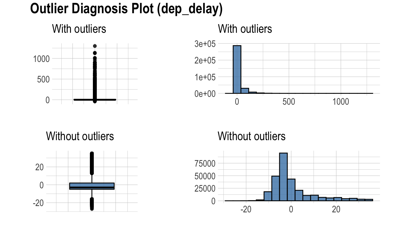
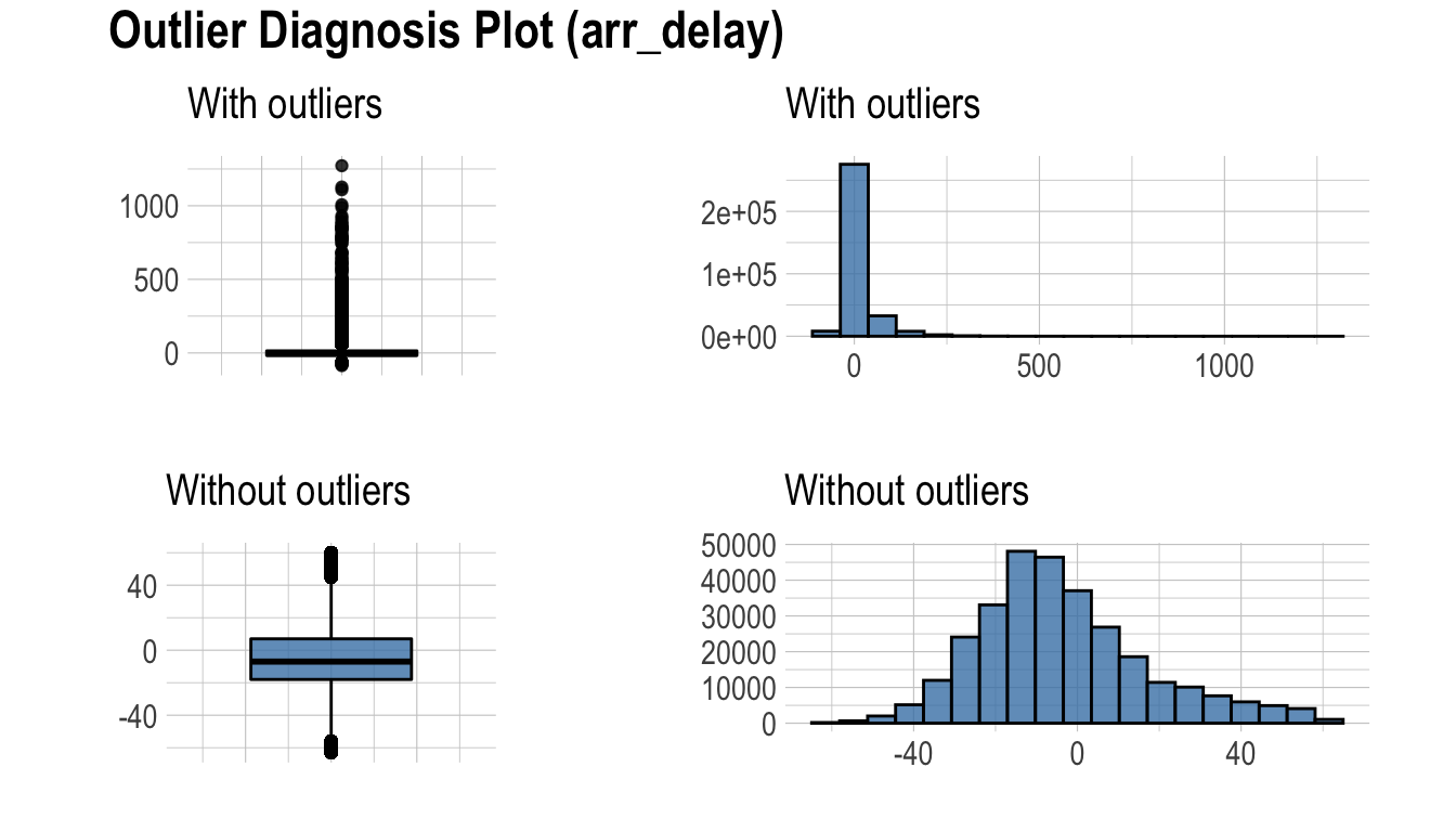
시각화 결과를 보고 이상치의 제거 및 대체 여부를 결정해야 한다. 경우에 따라서는 이상치가 포함된 변수를 데이터 분석 모델에서 제거하는 것도 고려해야 한다.
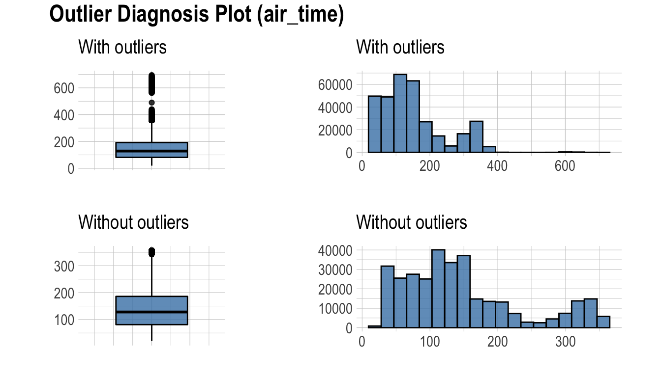
시각화 결과를 보면 arr_delay는 이상치를 제거한 관측치들은 정규분포와 유사한 분포를 보이고 있다. 선형 모형의 경우에는 이상치를 제거하거나 대체하는 것도 검토해볼 수 있겠다. 그리고 air_time은 이상치를 제거하기 전후의 분포가 대략 비슷한 모양을 보인다.
탐색적 데이터 분석
datasets
dlookr 패키지로 EDA를 수행하는 기초적인 사용 방법을 설명하기 위해서 Carseats를 사용한다. ISLR 패키지의 Carseats는 400개의 매장에서 아동용 카시트를 판매하는 시뮬레이션 데이터다. 이 데이터는 판매량을 예측하는 목적으로 생성한 데이터 프레임이다.
'data.frame':   400 obs. of  11 variables:
 $ Sales      : num  9.5 11.22 10.06 7.4 4.15 ...
 $ CompPrice  : num  138 111 113 117 141 124 115 136 132 132 ...
 $ Income     : num  73 48 35 100 64 113 105 81 110 113 ...
 $ Advertising: num  11 16 10 4 3 13 0 15 0 0 ...
 $ Population : num  276 260 269 466 340 501 45 425 108 131 ...
 $ Price      : num  120 83 80 97 128 72 108 120 124 124 ...
 $ ShelveLoc  : Factor w/ 3 levels "Bad","Good","Medium": 1 2 3 3 1 1 3 2 3 3 ...
 $ Age        : num  42 65 59 55 38 78 71 67 76 76 ...
 $ Education  : num  17 10 12 14 13 16 15 10 10 17 ...
 $ Urban      : Factor w/ 2 levels "No","Yes": 2 2 2 2 2 1 2 2 1 1 ...
 $ US         : Factor w/ 2 levels "No","Yes": 2 2 2 2 1 2 1 2 1 2 ...
개별 변수들의 의미는 다음과 같다. (ISLR::Carseats Man page 참고)
- Sales
- 지역의 단위 판매량 (단위: 천개)
- CompPrice
- 지역의 경쟁 업체가 부과하는 가격
- Income
- 지역 공동체 수입 수준 (단위: 천달러)
- Advertising
- 회사의 지역에 대한 광고 예산 (단위: 천달러)
- Population
- 지역의 인구 규모 (단위: 천명)
- Price
- 지역의 자동차 좌석 요금
- ShelveLoc
- 각 사이트에서 자동차 좌석의 선반 위치의 품질을 나타내는 수준. “Bad”, “Good”, “Medium”.
- Age
- 각 지역의 평균 연령
- Education
- 각 지역의 교육 수준
- Urban
- 점포의 도시 또는 농촌 소재 여부. Yes는 도시, No는 농촌.
- US
- 점포의 미국 소재 여부. Yes는 미국 소재, No는 미국 외 소재.
데이터 분석을 수행할 때, 결측치가 포함된 데이터를 자주 접한다. 그러나 Carseats는 결측치가 없은 완전한 데이터다. 그래서 다음과 같이 결측치를 생성하였다. 그리고 carseats라는 이름의 데이터 프레임 객체를 생성한다.
단변량 데이터 EDA
describe()을 이용한 기술통계량 계산
describe()는 수치 데이터의 기술통계량을 계산해 준다. 기술통계량은 수치 변수의 분포를 판단하는 것을 도와준다.
describe()가 반환하는 tbl_df 객체의 변수는 다음과 같다.
n: 결측치를 제외한 데이터 건수na: 결측치 건수mean: 산술평균sd: 표준편차se_mean: 표준오차. sd/sqrt(n)IQR: 사분위 범위(Interquartile range) (Q3-Q1)skewness: 왜도kurtosis: 첨도p25: Q1. 25% 백분위수p50: 중위수. 50% 백분위수p75: Q3. 75% 백분위수p01,p05,p10,p20,p30` : 1%, 5%, 20%, 30% 백분위수p40,p60,p70,p80` : 40%, 60%, 70%, 80% 백분위수p90,p95,p99,p100` : 90%, 95%, 99%, 100% 백분위수
다음처럼 describe()는 carseats의 모든 수치 변수의 통계량을 계산한다.:
describe(carseats)
# A tibble: 8 x 26
  variable      n    na   mean     sd se_mean    IQR skewness kurtosis
  <chr>     <int> <int>  <dbl>  <dbl>   <dbl>  <dbl>    <dbl>    <dbl>
1 Sales       400     0   7.50   2.82   0.141   3.93   0.186   -0.0809
2 CompPrice   400     0 125.    15.3    0.767  20     -0.0428   0.0417
3 Income      380    20  69.3   28.1    1.44   48      0.0360  -1.10
4 Advertis…   400     0   6.64   6.65   0.333  12      0.640   -0.545
5 Populati…   400     0 265.   147.     7.37  260.    -0.0512  -1.20
6 Price       400     0 116.    23.7    1.18   31     -0.125    0.452
7 Age         400     0  53.3   16.2    0.810  26.2   -0.0772  -1.13
8 Education   400     0  13.9    2.62   0.131   4      0.0440  -1.30
# … with 17 more variables: p00 <dbl>, p01 <dbl>, p05 <dbl>,
#   p10 <dbl>, p20 <dbl>, p25 <dbl>, p30 <dbl>, p40 <dbl>, p50 <dbl>,
#   p60 <dbl>, p70 <dbl>, p75 <dbl>, p80 <dbl>, p90 <dbl>, p95 <dbl>,
# p99 <dbl>, p100 <dbl>왜도: 왼쪽으로 치우친 분포의 데이터, 즉 skewness가 제법 큰 양수를 갖는 변수는 정규분포를 따르도록 log, sqrt 변환 등을 고려해야 한다. Advertising 변수는 변수변환을 고려해야할 것 같다.산술평균,표준편차,표준오차: 표준오차(se_mean)가 7.3688218로 상당히 큰Population는 대표치인 산술평균(mean)의 대표성이 낮다. 산술평균에 비해서 표준편차(sd)의 크기도 상당히 큰 편이다.
dplyr을 이용해서 왼쪽이나 오른쪽으로 치우친 정도(왜도)의 크기별로 정렬할 수 있다.:
carseats %>%
  describe() %>%
  select(variable, skewness, mean, p25, p50, p75) %>%
  filter(!is.na(skewness)) %>%
  arrange(desc(abs(skewness)))
# A tibble: 8 x 6
  variable    skewness   mean    p25    p50    p75
  <chr>          <dbl>  <dbl>  <dbl>  <dbl>  <dbl>
1 Advertising   0.640    6.64   0      5     12
2 Sales         0.186    7.50   5.39   7.49   9.32
3 Price        -0.125  116.   100    117    131
4 Age          -0.0772  53.3   39.8   54.5   66
5 Population   -0.0512 265.   139    272    398.
6 Education     0.0440  13.9   12     14     16
7 CompPrice    -0.0428 125.   115    125    135
8 Income        0.0360  69.3   44     69     92
describe() 함수는 dplyr 패키지의 group_by() 함수 구문을 지원한다.
# A tibble: 12 x 28
   variable US    Urban     n    na  mean    sd se_mean   IQR skewness
   <chr>    <fct> <fct> <int> <int> <dbl> <dbl>   <dbl> <dbl>    <dbl>
 1 Income   No    No       40     4 62.1  29.8    4.72  51.8    0.367
 2 Income   No    Yes      91     3 67.5  27.4    2.87  48      0.0518
 3 Income   No    <NA>      3     1 59.7  37.0   21.4   37     -0.162
 4 Income   Yes   No       68     3 70.2  30.7    3.72  53      0.0414
 5 Income   Yes   Yes     172     9 71.4  26.5    2.02  45     -0.0201
 6 Income   Yes   <NA>      6     0 79.8  34.9   14.3   53.5   -0.506
 7 Sales    No    No       44     0  6.42  2.78   0.418  3.29   0.132
 8 Sales    No    Yes      94     0  7.00  2.56   0.264  3.49   0.491
 9 Sales    No    <NA>      4     0  7.04  1.04   0.518  1.26  -0.887
10 Sales    Yes   No       71     0  8.21  2.61   0.310  4.08  -0.0453
11 Sales    Yes   Yes     181     0  7.77  2.95   0.219  3.99   0.134
12 Sales    Yes   <NA>      6     0  6.84  3.70   1.51   4.87   0.599
# … with 18 more variables: kurtosis <dbl>, p00 <dbl>, p01 <dbl>,
#   p05 <dbl>, p10 <dbl>, p20 <dbl>, p25 <dbl>, p30 <dbl>, p40 <dbl>,
#   p50 <dbl>, p60 <dbl>, p70 <dbl>, p75 <dbl>, p80 <dbl>, p90 <dbl>,
# p95 <dbl>, p99 <dbl>, p100 <dbl>normality()을 이용한 수치형 변수의 정규성 검정
normality()는 수치 데이터의 정규성 검정을 수행한다. Shapiro-Wilk 정규성 검정을 수행하며, 관측치의 개수가 5000보다 클 경우에는 5000개의 단순 임의 추출을 수행한 후 검정한다.
normality()가 반환하는 tbl_df 객체의 변수는 다음과 같다.
statistic: Shapiro-Wilk 검정의 통계량p_value: Shapiro-Wilk 검정의 p-valuesample: Shapiro-Wilk 검정을 수행한 샘플 관측치의 개수
다음처럼 normality()는 carseats의 모든 수치 변수의 정규성 검정을 수행한다.:
normality(carseats)
# A tibble: 8 x 4
  vars        statistic  p_value sample
  <chr>           <dbl>    <dbl>  <dbl>
1 Sales           0.995 2.54e- 1    400
2 CompPrice       0.998 9.77e- 1    400
3 Income          0.961 1.55e- 8    400
4 Advertising     0.874 1.49e-17    400
5 Population      0.952 4.08e-10    400
6 Price           0.996 3.90e- 1    400
7 Age             0.957 1.86e- 9    400
8 Education       0.924 2.43e-13    400
dplyr을 이용해서 정규분포를 따르지 않는 변수를 p_value 순으로 정렬할 수 있다.:
# A tibble: 5 x 4
  vars        statistic  p_value sample
  <chr>           <dbl>    <dbl>  <dbl>
1 Advertising     0.874 1.49e-17    400
2 Education       0.924 2.43e-13    400
3 Population      0.952 4.08e-10    400
4 Age             0.957 1.86e- 9    400
5 Income          0.961 1.55e- 8    400
특히 Advertising 변수는 정규분포에서 가장 벗어난 것으로 파악된다.
normality() 함수는 dplyr 패키지의 group_by() 함수 구문을 지원한다.
# A tibble: 6 x 6
  variable ShelveLoc US    statistic p_value sample
  <chr>    <fct>     <fct>     <dbl>   <dbl>  <dbl>
1 Income   Bad       No        0.965 0.350       34
2 Income   Good      Yes       0.958 0.0359      61
3 Income   Bad       Yes       0.952 0.0236      62
4 Income   Good      No        0.879 0.0140      24
5 Income   Medium    Yes       0.964 0.00190    135
6 Income   Medium    No        0.944 0.00161     84
Income 변수는 정규분포를 따르지 않지만, 유의수준 0.01 기준으로 US가 No이면서 ShelveLoc가 Good, Bad인 경우는 정규분포를 따르는 것으로 볼 수 있다.
다음은 범주형 변수인 ShelveLoc, US 변수의 조합별로 log(Income)의 정규성 검정을 수행하여, 정규분포를 따르는 변수를 조회한다.
carseats %>%
  mutate(log_income = log(Income)) %>%
  group_by(ShelveLoc, US) %>%
  normality(log_income) %>%
  filter(p_value > 0.01)
# A tibble: 1 x 6
variable ShelveLoc US statistic p_value sample
<chr> <fct> <fct> <dbl> <dbl> <dbl>
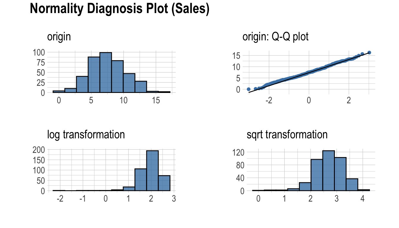
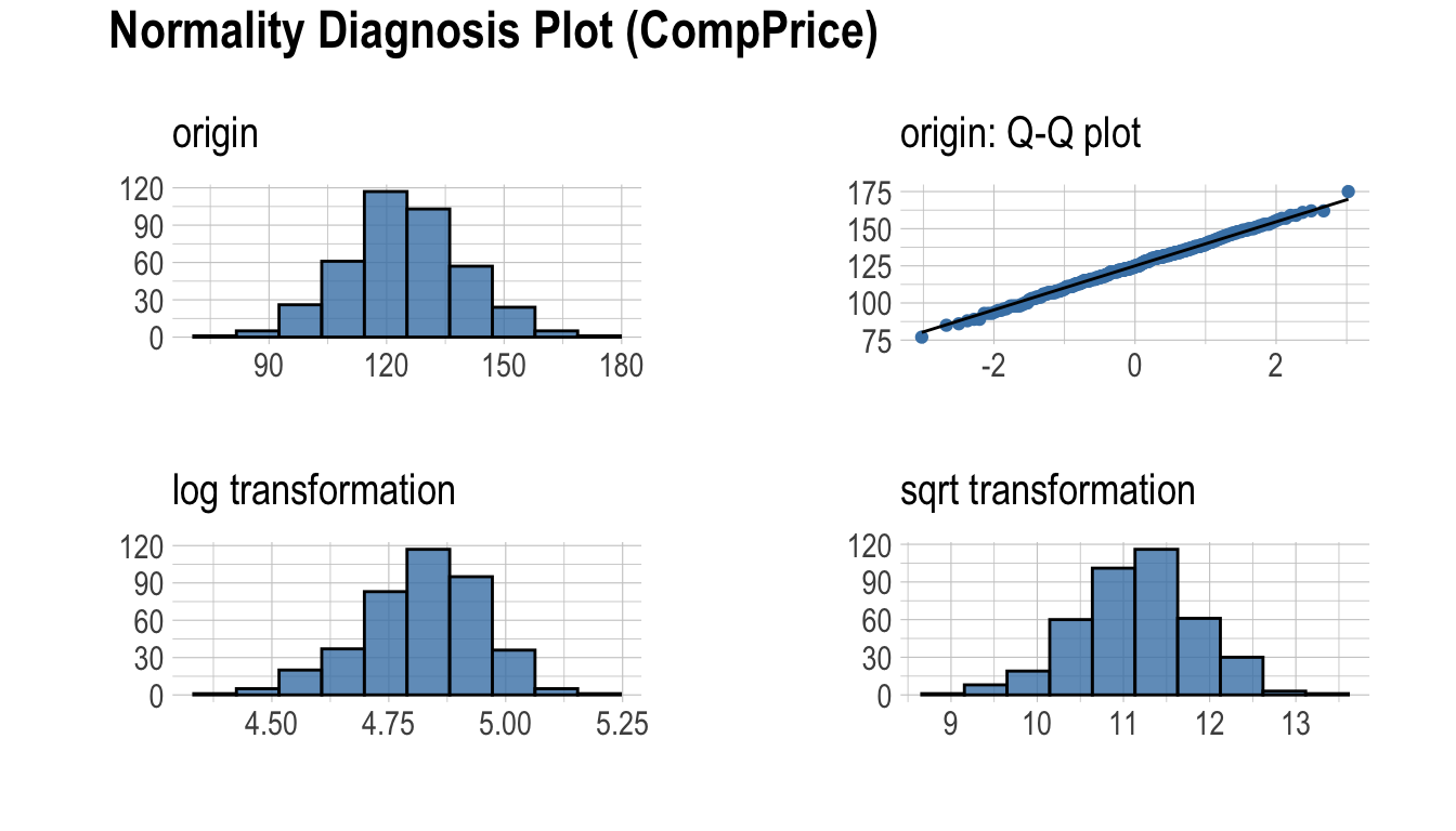
1 log_income Bad No 0.946 0.100 34plot_normality()를 이용한 수치변수의 정규성 시각화
plot_normality()는 수치 데이터의 정규성을 시각화한다.
plot_normality()가 시각화하는 정보는 다음과 같다.
원 데이터의 히스토그램원 데이터의 Q-Q plotlog 변환 데이터의 히스토그램sqrt 변환 데이터의 히스토그램
데이터 분석 과정에서 멱분포(power-law distribution)를 따르는 수치 데이터를 접하는 경우가 많다. 멱분포를 따르는 수치 데이터는 log, sqrt 변환을 수행하여 정규분포로 변화라기 때문에 log, sqrt 변환데 데이터의 히스토그램을 그린다.
plot_normality()도 normality() 함수처럼 여러 개의 변수를 지정할 수 있다.
# Select columns by name
plot_normality(carseats, Sales, CompPrice)
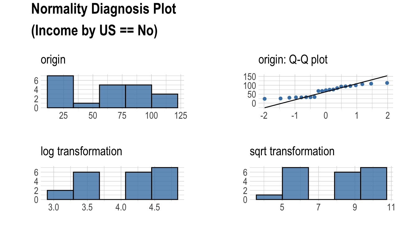
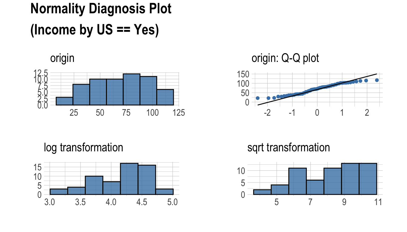
plot_normality() 함수도 dplyr 패키지의 group_by() 함수 구문을 지원한다.
carseats %>%
  filter(ShelveLoc == "Good") %>%
  group_by(US) %>%
  plot_normality(Income)
이변량 데이터 EDA
correlate()을 이용한 상관계수 계산
다음처럼 correlate()는 carseats의 모든 수치 변수의 조합의 상관계수를 구한다.:
correlate(carseats)
# A tibble: 56 x 3
   var1        var2      coef_corr
   <fct>       <fct>         <dbl>
 1 CompPrice   Sales        0.0641
 2 Income      Sales        0.153
 3 Advertising Sales        0.270
 4 Population  Sales        0.0505
 5 Price       Sales       -0.445
 6 Age         Sales       -0.232
 7 Education   Sales       -0.0520
 8 Sales       CompPrice    0.0641
 9 Income      CompPrice   -0.0918
10 Advertising CompPrice   -0.0242
# … with 46 more rows
다음은 선택된 몇 개의 변수를 포함한 조합에 대해서만 정규성 검정을 수행한다.
# Select columns by name
correlate(carseats, Sales, CompPrice, Income)
# A tibble: 21 x 3
   var1      var2        coef_corr
   <fct>     <fct>           <dbl>
 1 CompPrice Sales          0.0641
 2 Income    Sales          0.153
 3 Sales     CompPrice      0.0641
 4 Income    CompPrice     -0.0918
 5 Sales     Income         0.153
 6 CompPrice Income        -0.0918
 7 Sales     Advertising    0.270
 8 CompPrice Advertising   -0.0242
 9 Income    Advertising    0.0674
10 Sales     Population     0.0505
# … with 11 more rowscorrelate()는 두벌의 변수 조합을 만든다. 그래서 다음과 같은 filter() 함수를 사용해서 한 벌의 조합에 대한 상관계수를 구할 수 있다.:
carseats %>%
  correlate(Sales:Income) %>%
  filter(as.integer(var1) > as.integer(var2))
# A tibble: 3 x 3
  var1      var2      coef_corr
  <fct>     <fct>         <dbl>
1 CompPrice Sales        0.0641
2 Income    Sales        0.153
3 Income    CompPrice   -0.0918
correlate() 함수도 dplyr 패키지의 group_by() 함수 구문을 지원한다.
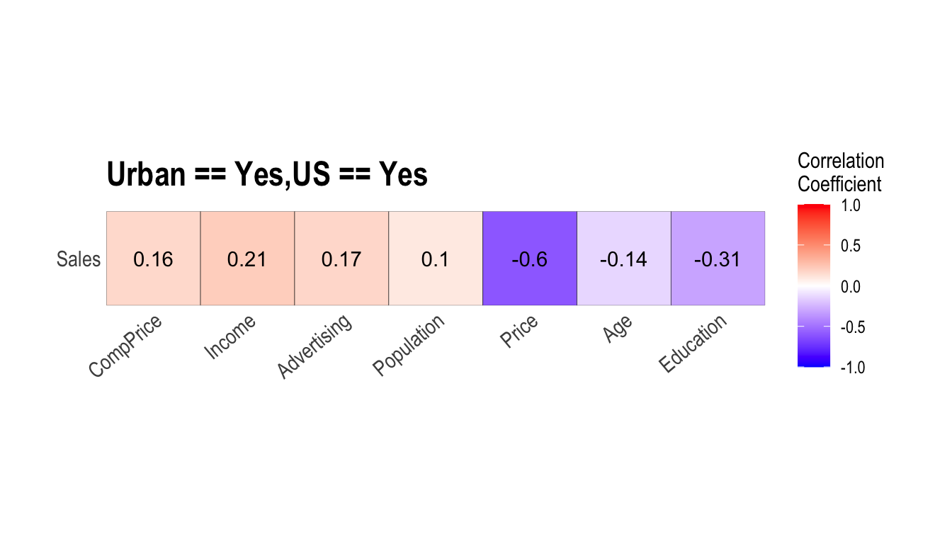
carseats %>%
  filter(ShelveLoc == "Good") %>%
  group_by(Urban, US) %>%
  correlate(Sales) %>%
  filter(abs(coef_corr) > 0.5)
# A tibble: 6 x 5
Urban US var1 var2 coef_corr
<fct> <fct> <fct> <fct> <dbl>
1 No No Sales Population -0.530
2 No No Sales Price -0.838
3 No Yes Sales Price -0.655
4 Yes No Sales Price -0.837
5 Yes No Sales Age -0.644
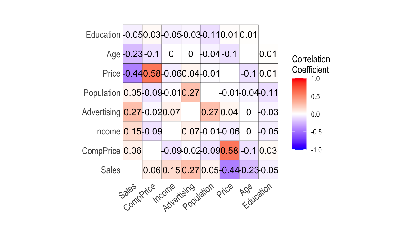
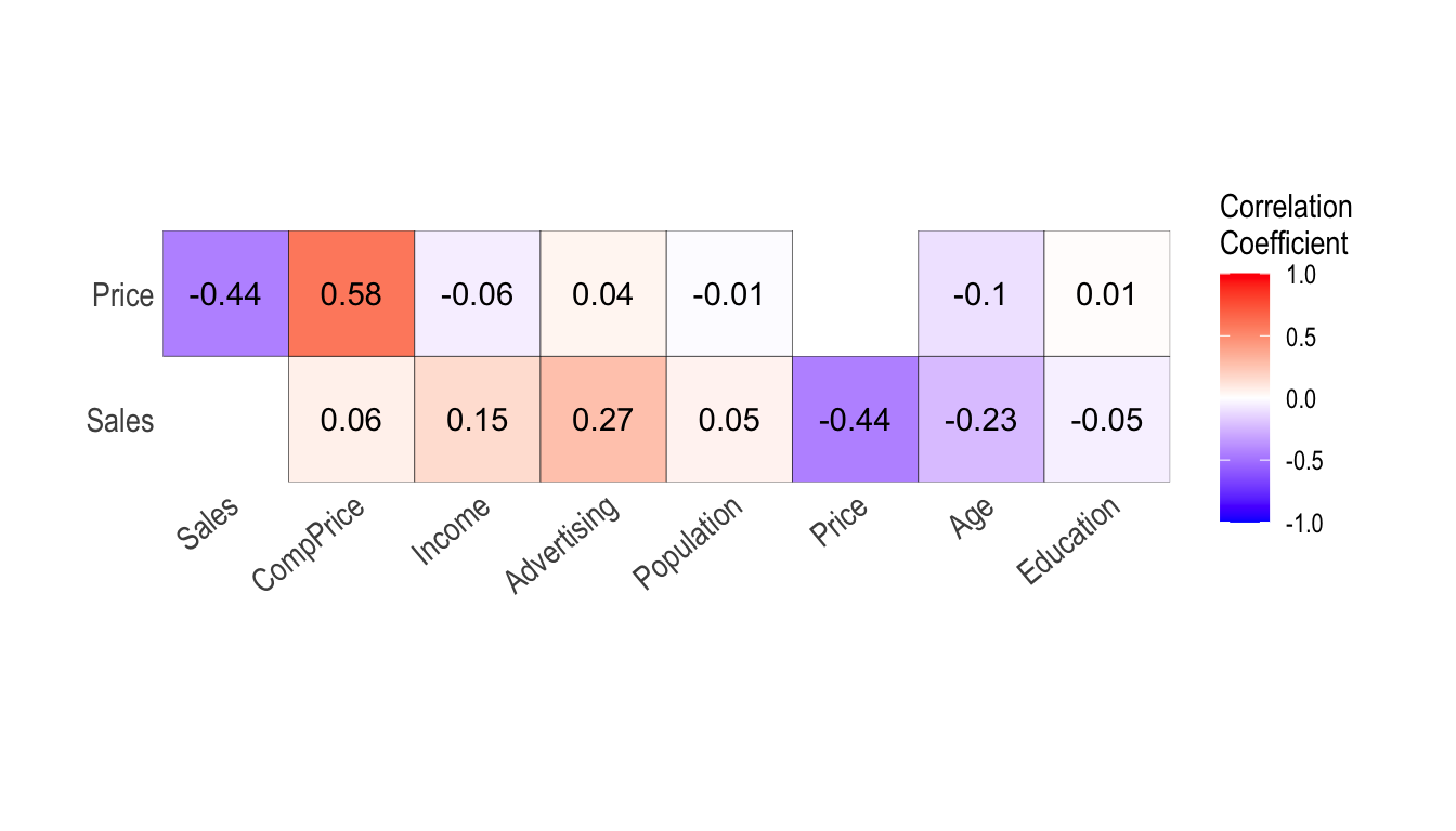
6 Yes Yes Sales Price -0.604plot_correlate()를 이용한 상관행렬의 시각화
plot_correlate()는 상관행렬을 시각화한다.
plot_correlate(carseats)
plot_correlate()도 correlate() 함수처럼 여러 개의 변수를 지정할 수 있다.
다음은 선택된 몇 개의 변수를 포함한 상관행렬의 시각화를 수행한다.
# Select columns by name
plot_correlate(carseats, Sales, Price)
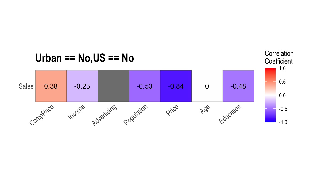
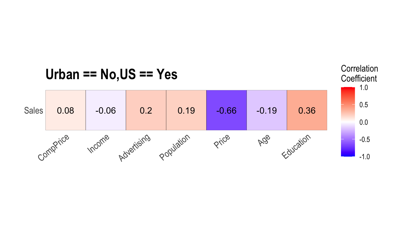
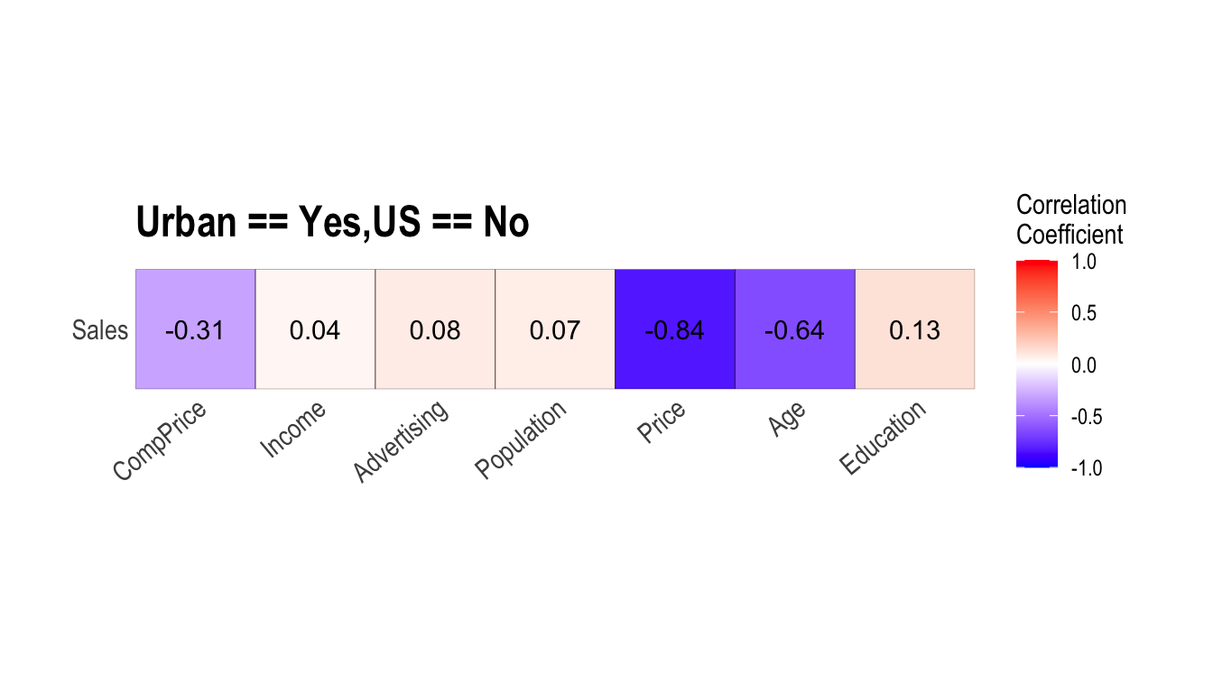
plot_correlate() 함수도 dplyr 패키지의 group_by() 함수 구문을 지원한다.
carseats %>%
  filter(ShelveLoc == "Good") %>%
  group_by(Urban, US) %>%
  plot_correlate(Sales)
Target 변수에 기반한 EDA
Target 변수 정의
Target 변수 기반으로 EDA를 수행하려면 target_by 클래스 객체를 생성해야 한다. target_by()는 data.frame 또는 data.frame을 상속받은 객체로 target_by 클래스를 생성한다. target_by()는 grouped_df를 생성하는 dplyr의 group_by()와 유사하다. 차이점은 하나의 변수만 지정한다는 것이다.
다음은 carseats data.frame에서 US를 target 변수로 지정하는 예제다.:
categ <- target_by(carseats, US)
Target 변수가 범주형 변수인 경우의 EDA
Target 변수가 범주형일 때 EDA를 수행해 보자. 범주형 변수 US가 target 변수일 때, target 변수와 예측 변수(Predictor) 사이의 관계를 살펴본다.
예측변수가 수치형 변수인 경우
relate()는 taregt 변수와 예측변수 사이의 관계를 보여준다. 다음 예제는 예측변수 Sales와 target 변수 US 사이의 관계를 보여준다. 예측변수 Sales는 수치형 변수다. 이 경우, target 변수의 각 레벨에 대한 기술통계(descriptive statistics)가 표현된다.
# If the variable of interest is a numarical variable
cat_num <- relate(categ, Sales)
cat_num
# A tibble: 3 x 27
  variable US        n    na  mean    sd se_mean   IQR skewness
  <chr>    <fct> <int> <int> <dbl> <dbl>   <dbl> <dbl>    <dbl>
1 Sales    No      142     0  6.82  2.60   0.218  3.44   0.323
2 Sales    Yes     258     0  7.87  2.88   0.179  4.23   0.0760
3 Sales    total   400     0  7.50  2.82   0.141  3.93   0.186
# … with 18 more variables: kurtosis <dbl>, p00 <dbl>, p01 <dbl>,
#   p05 <dbl>, p10 <dbl>, p20 <dbl>, p25 <dbl>, p30 <dbl>, p40 <dbl>,
#   p50 <dbl>, p60 <dbl>, p70 <dbl>, p75 <dbl>, p80 <dbl>, p90 <dbl>,
# p95 <dbl>, p99 <dbl>, p100 <dbl>summary(cat_num)
   variable             US          n               na
 Length:3           No   :1   Min.   :142.0   Min.   :0
 Class :character   Yes  :1   1st Qu.:200.0   1st Qu.:0
 Mode  :character   total:1   Median :258.0   Median :0
                              Mean   :266.7   Mean   :0
                              3rd Qu.:329.0   3rd Qu.:0
                              Max.   :400.0   Max.   :0
      mean             sd           se_mean            IQR
 Min.   :6.823   Min.   :2.603   Min.   :0.1412   Min.   :3.442
 1st Qu.:7.160   1st Qu.:2.713   1st Qu.:0.1602   1st Qu.:3.686
 Median :7.496   Median :2.824   Median :0.1791   Median :3.930
 Mean   :7.395   Mean   :2.768   Mean   :0.1796   Mean   :3.866
 3rd Qu.:7.682   3rd Qu.:2.851   3rd Qu.:0.1988   3rd Qu.:4.077
 Max.   :7.867   Max.   :2.877   Max.   :0.2184   Max.   :4.225
    skewness          kurtosis             p00
 Min.   :0.07603   Min.   :-0.32638   Min.   :0.0000
 1st Qu.:0.13080   1st Qu.:-0.20363   1st Qu.:0.0000
 Median :0.18556   Median :-0.08088   Median :0.0000
 Mean   :0.19489   Mean   : 0.13350   Mean   :0.1233
 3rd Qu.:0.25432   3rd Qu.: 0.36344   3rd Qu.:0.1850
 Max.   :0.32308   Max.   : 0.80776   Max.   :0.3700
      p01              p05             p10             p20
 Min.   :0.4675   Min.   :3.147   Min.   :3.917   Min.   :4.754
 1st Qu.:0.6868   1st Qu.:3.148   1st Qu.:4.018   1st Qu.:4.910
 Median :0.9062   Median :3.149   Median :4.119   Median :5.066
 Mean   :1.0072   Mean   :3.183   Mean   :4.073   Mean   :5.051
 3rd Qu.:1.2771   3rd Qu.:3.200   3rd Qu.:4.152   3rd Qu.:5.199
 Max.   :1.6480   Max.   :3.252   Max.   :4.184   Max.   :5.332
      p25             p30             p40             p50
 Min.   :5.080   Min.   :5.306   Min.   :5.994   Min.   :6.660
 1st Qu.:5.235   1st Qu.:5.587   1st Qu.:6.301   1st Qu.:7.075
 Median :5.390   Median :5.867   Median :6.608   Median :7.490
 Mean   :5.411   Mean   :5.775   Mean   :6.506   Mean   :7.313
 3rd Qu.:5.576   3rd Qu.:6.010   3rd Qu.:6.762   3rd Qu.:7.640
 Max.   :5.763   Max.   :6.153   Max.   :6.916   Max.   :7.790
      p60             p70             p75             p80
 Min.   :7.496   Min.   :7.957   Min.   :8.523   Min.   : 8.772
 1st Qu.:7.787   1st Qu.:8.386   1st Qu.:8.921   1st Qu.: 9.265
 Median :8.078   Median :8.815   Median :9.320   Median : 9.758
 Mean   :8.076   Mean   :8.740   Mean   :9.277   Mean   : 9.665
 3rd Qu.:8.366   3rd Qu.:9.132   3rd Qu.:9.654   3rd Qu.:10.111
 Max.   :8.654   Max.   :9.449   Max.   :9.988   Max.   :10.464
      p90              p95             p99             p100
 Min.   : 9.349   Min.   :11.28   Min.   :13.64   Min.   :14.90
 1st Qu.:10.325   1st Qu.:11.86   1st Qu.:13.78   1st Qu.:15.59
 Median :11.300   Median :12.44   Median :13.91   Median :16.27
 Mean   :10.795   Mean   :12.08   Mean   :13.86   Mean   :15.81
 3rd Qu.:11.518   3rd Qu.:12.49   3rd Qu.:13.97   3rd Qu.:16.27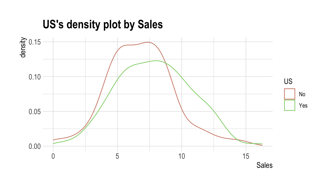
Max. :11.736 Max. :12.54 Max. :14.03 Max. :16.27 relate()로 생성된 relate 클래스 객체를, plot ()으로 target 변수와 예측변수 사이의 관계를 시각화한다. US와 Sales 간의 관계는 밀도 플롯(density plot)으로 표현된다.
plot(cat_num)
예측변수가 범주형 변수인 경우
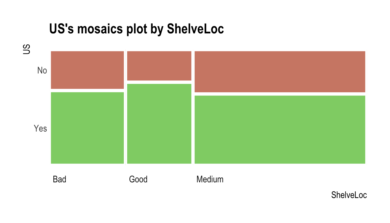
다음 예제는 ShelveLoc과 target 변수 US 사이의 관계를 보여준다. 예측변수인 ShelveLoc는 범주형 변수다. 이 경우는 두 변수의 분할표(contentency table)를 보여준다. summary() 함수는 분할표에 대해 독립성 검정을 수행한다.
# If the variable of interest is a categorical variable
cat_cat <- relate(categ, ShelveLoc)
cat_cat
     ShelveLoc
US    Bad Good Medium
  No   34   24     84
Yes 62 61 135summary(cat_cat)
Call: xtabs(formula = formula_str, data = data, addNA = TRUE)
Number of cases in table: 400
Number of factors: 2
Test for independence of all factors:
Chisq = 2.7397, df = 2, p-value = 0.2541plot()은 target 변수와 예측변수 사이의 관계를 시각화한다. US와 ShelveLoc 사이의 관계는 모자이크 플롯(mosaics plot)으로 표현된다.
plot(cat_cat)
Target 변수가 수치형 변수일 때의 EDA
Target 변수가 수치형일 때 EDA를 수행해 보자. 수치형 변수 `Sales가 target 변수일 때, target 변수와 예측 변수(Predictor) 사이의 관계를 살펴본다.
# If the variable of interest is a numarical variable
num <- target_by(carseats, Sales)
예측변수가 수치형 변수인 경우
다음 예제는 Price와 target 변수 Sales 사이의 관계를 보여준다. 예측변수인 Price는 수치형 변수다. 이 경우, target ~ predictor 관계의 단순 회귀 모델(simple linear model)의 결과를 보여준다. summary() 함수는 모델의 세부 사항을 표현한다.
# If the variable of interest is a numarical variable
num_num <- relate(num, Price)
num_num
Call:
lm(formula = formula_str, data = data)

Coefficients:
(Intercept)        Price
13.64192 -0.05307 summary(num_num)
Call:
lm(formula = formula_str, data = data)

Residuals:
    Min      1Q  Median      3Q     Max
-6.5224 -1.8442 -0.1459  1.6503  7.5108

Coefficients:
             Estimate Std. Error t value Pr(>|t|)
(Intercept) 13.641915   0.632812  21.558   <2e-16 ***
Price       -0.053073   0.005354  -9.912   <2e-16 ***
---
Signif. codes:  0 '***' 0.001 '**' 0.01 '*' 0.05 '.' 0.1 ' ' 1

Residual standard error: 2.532 on 398 degrees of freedom
Multiple R-squared:  0.198, Adjusted R-squared:  0.196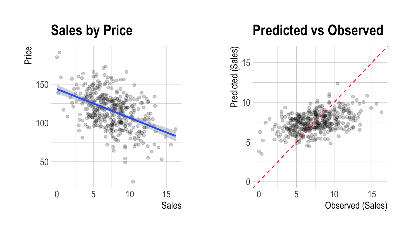
F-statistic: 98.25 on 1 and 398 DF, p-value: < 2.2e-16plot()은 target 변수와 예측변수 사이의 관계를 시각화한다. Sales와 Price 간의 관계는 산점도(scatter plot)로 시각화된다. 왼쪽 그림은 Sales와 Price의 산포도와 회귀선 및 회귀선의 신뢰구간을 나타낸다. 오른쪽 그림은 원 데이터와 선형모델의 예측값 사이의 관계를 산점도로 나타낸 것이다. 두 변수 사이에 선형 관계가 있는 경우 관측치의 산점도는 빨간색 대각선에 수렴한다.
plot(num_num)
예측변수가 범주형 변수인 경우
다음 예제는 ShelveLoc과 target 변수 Sales 사이의 관계를 보여준다. 예측변수인 ShelveLoc은 범주형 변수다. target-predictor 관계의 one-way ANOVA를 수행한 결과를 보여준다. 결과는 분산분석의 관점에서 표현된다. summary() 함수는 예측변수의 각 레벨에 대한 회귀 계수를 보여준다. 다시말해 target ~ predictor 관계의 단순 회귀분석에 대한 상세 정보를 보여준다.
# If the variable of interest is a categorical variable
num_cat <- relate(num, ShelveLoc)
num_cat
Analysis of Variance Table

Response: Sales
           Df Sum Sq Mean Sq F value    Pr(>F)
ShelveLoc   2 1009.5  504.77   92.23 < 2.2e-16 ***
Residuals 397 2172.7    5.47
---
Signif. codes: 0 '***' 0.001 '**' 0.01 '*' 0.05 '.' 0.1 ' ' 1summary(num_cat)
Call:
lm(formula = formula(formula_str), data = data)
Residuals:
Min 1Q Median 3Q Max
-7.3066 -1.6282 -0.0416 1.5666 6.1471
Coefficients:
Estimate Std. Error t value Pr(>|t|)
(Intercept) 5.5229 0.2388 23.131 < 2e-16 ***
ShelveLocGood 4.6911 0.3484 13.464 < 2e-16 ***
ShelveLocMedium 1.7837 0.2864 6.229 1.2e-09 ***
---
Signif. codes: 0 '***' 0.001 '**' 0.01 '*' 0.05 '.' 0.1 ' ' 1
Residual standard error: 2.339 on 397 degrees of freedom
Multiple R-squared: 0.3172, Adjusted R-squared: 0.3138
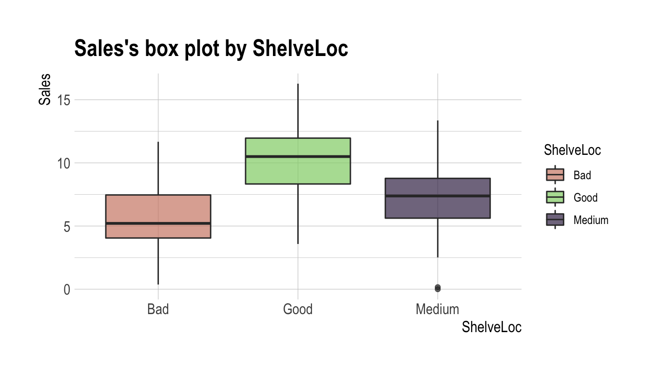
F-statistic: 92.23 on 2 and 397 DF, p-value: < 2.2e-16plot ()은 target 변수와 예측변수 사이의 관계를 시각화한다. Sales와 ShelveLoc의 관계는 박스플롯(box plot)으로 표현된다.
plot(num_cat)
데이터 변환
dlookr은 결측치와 이상치의 대체, 치우친 데이터를 보정해준다. 또한 연속형 변수를 범주형 변수로 비닝하는 것을 도와준다.
다음은 dlookr이 제공하는 데이터 변환 함수와 함수의 기능 목록이다.:
find_na()는 결측치가 포함된 변수를 찾아주고,imputate_na()는 결측치를 대체한다.find_outliers()는 이상치가 포함된 변수를 찾아주고,imputate_outlier()는 이상치를 대체한다.summary.imputation()와plot.imputation()는 대체된 변수의 정보를 보혀주고 시각화를 제공한다.find_skewness()는 치우친 데이터의 변수를 찾아주고,transform()는 치우친 데이터의 보정을 수행한다.- 또한
transform()는 수치형 변수의 표준화를 수행한다. summary.transform()와plot.transform()는 변환된 변수의 정보를 보혀주고 시각화를 제공한다.binning()와binning_by()는 수치 데이터를 비닝하여 범주형 데이터로 변환한다.print.bins()와summary.bins()는 비닝 결과를 보여주고 요약해 준다.plot.bins()와plot.optimal_bins()는 비닝 결과의 시각화를 제공한다.transformation_report()는 데이터 변환을 수행한 후 그 결과를 보고서로 만들어 준다.
결측치의 대체
imputate_na()을 이용한 결측치의 대체
imputate_na()는 변수에 포함된 결측치를 대체한다. 결측치가 포함된 예측변수(predictor)는 수치형 변수와 범주형 변수 모두 지원하며, 다음과 같은 method를 지원한다.
- predictor가 수치형 변수일 경우
- “mean” : 산술평균으로 대체
- “median” : 중위수로 대체
- “mode” : 최빈수로 대체
- “knn” : K-nearest neighbors를 이용한 대체
- target 변수를 지정해야 함
- “rpart” : Recursive Partitioning and Regression Trees를 이용한 대체
- target 변수를 지정해야 함
- target 변수를 지정해야 함
- “mice” : Multivariate Imputation by Chained Equations를 이용한 대체
- target 변수를 지정해야 함
- random seed를 지정해야 함
- predictor가 범주형 변수일 경우
- “mode” : 최빈수로 대체
- “rpart” : Recursive Partitioning and Regression Trees를 이용한 대체
- target 변수를 지정해야 함
- target 변수를 지정해야 함
- “mice” : Multivariate Imputation by Chained Equations를 이용한 대체
- target 변수를 지정해야 함
- random seed를 지정해야 함
- target 변수를 지정해야 함
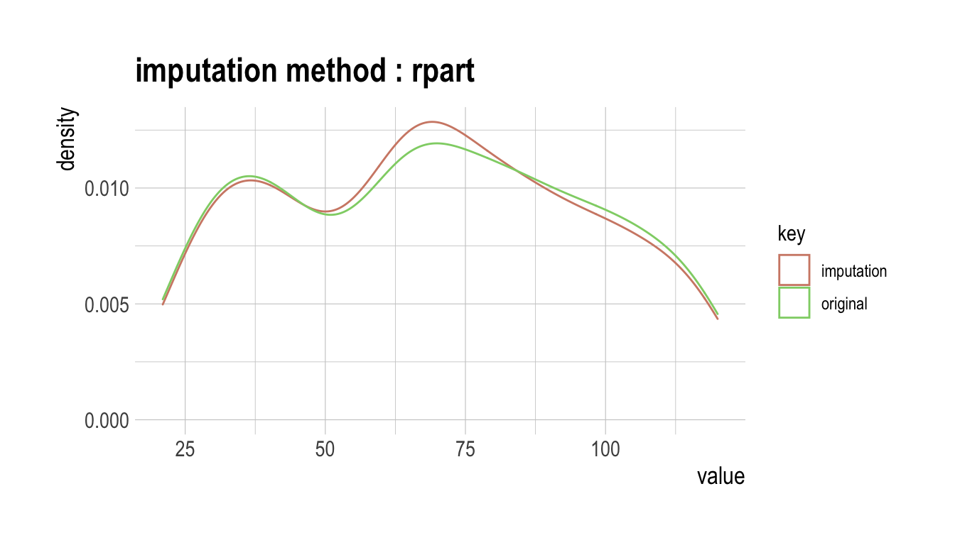
다음처럼 imputate_na()는 carseats의 수치형 변수인 Income를 “rpart” 방법으로 결측치를 대체한다. summary()는 결측치 대체 정보를 요약하고, plot()은 결측정보를 시각화한다.
income <- imputate_na(carseats, Income, US, method = "rpart")

# result of imputate
income
  [1]  73.00000  48.00000  35.00000 100.00000  64.00000 113.00000
  [7] 105.00000  81.00000 110.00000 113.00000  78.00000  94.00000
 [13]  35.00000  58.63636 117.00000  95.00000  32.00000  74.00000
 [19] 110.00000  76.00000  90.00000  29.00000  46.00000  31.00000
 [25] 119.00000  32.00000 115.00000 118.00000  74.00000  99.00000
 [31]  94.00000  58.00000  32.00000  38.00000  54.00000  84.00000
 [37]  76.00000  41.00000  73.00000  60.00000  98.00000  53.00000
 [43]  69.00000  42.00000  79.00000  63.00000  90.00000  98.00000
 [49]  52.00000  93.00000  32.00000  90.00000  40.00000  64.00000
 [55] 103.00000  81.00000  82.00000  91.00000  93.00000  71.00000
 [61] 102.00000  32.00000  45.00000  88.00000  67.00000  26.00000
 [67]  92.00000  61.00000  69.00000  59.00000  81.00000  51.00000
 [73]  45.00000  90.00000  68.00000 111.00000  87.00000  71.00000
 [79]  48.00000  67.00000 100.00000  72.00000  83.00000  36.00000
 [85]  25.00000 103.00000  84.00000  67.00000  42.00000  56.07143
 [91]  67.14286  46.00000 113.00000  30.00000  97.00000  25.00000
 [97]  42.00000  82.00000  77.00000  47.00000  69.00000  93.00000
[103]  22.00000  91.00000  96.00000 100.00000  33.00000 107.00000
[109]  79.00000  65.00000  62.00000 118.00000  99.00000  29.00000
[115]  87.00000  35.00000  75.00000  75.34722  88.00000  94.00000
[121] 105.00000  89.00000 100.00000 103.00000 113.00000  78.00000
[127]  68.00000  48.00000 100.00000 120.00000  84.00000  69.00000
[133]  87.00000  98.00000  31.00000  94.00000  68.81481  42.00000
[139] 103.00000  62.00000  60.00000  42.00000  84.00000  88.00000
[145]  68.00000  63.00000  83.00000  54.00000 119.00000 120.00000
[151]  84.00000  58.00000  67.77778  36.00000  69.00000  72.00000
[157]  34.00000  58.00000  90.00000  60.00000  28.00000  21.00000
[163]  74.00000  64.00000  64.00000  58.00000  67.00000  73.00000
[169]  89.00000  41.00000  39.00000 106.00000 102.00000  91.00000
[175]  24.00000  89.00000 107.00000  72.00000  89.86364  25.00000
[181] 112.00000  83.00000  60.00000  74.00000  33.00000 100.00000
[187]  51.00000  32.00000  37.00000 117.00000  37.00000  42.00000
[193]  26.00000  70.00000  56.07143  93.00000  65.50000  61.00000
[199]  80.00000  88.00000  92.00000  83.00000  78.00000  82.00000
[205]  80.00000  22.00000  67.00000 105.00000  54.00000  21.00000
[211]  41.00000 118.00000  69.00000  84.00000 115.00000  83.00000
[217]  33.00000  44.00000  61.00000  79.00000 120.00000  44.00000
[223] 119.00000  45.00000  82.00000  25.00000  33.00000  64.00000
[229]  67.50000 104.00000  60.00000  69.00000  80.00000  76.00000
[235]  62.00000  32.00000  34.00000  28.00000  24.00000 105.00000
[241]  80.00000  63.00000  46.00000  68.81481  30.00000  43.00000
[247]  56.00000 114.00000  52.00000  67.00000 105.00000 111.00000
[253]  97.00000  24.00000 104.00000  55.55556  40.00000  62.00000
[259]  38.00000  36.00000 117.00000  42.00000  77.00000  26.00000
[265]  29.00000  35.00000  93.00000  82.00000  57.00000  69.00000
[271]  26.00000  56.00000  33.00000 106.00000  93.00000 119.00000
[277]  69.00000  48.00000 113.00000  57.00000  86.00000  69.00000
[283]  96.00000 110.00000  46.00000  26.00000 118.00000  44.00000
[289]  40.00000  77.00000 111.00000  70.00000  66.00000  84.00000
[295]  76.00000  35.00000  44.00000  83.00000  75.34722  40.00000
[301]  78.00000  93.00000  77.00000  52.00000  98.00000  67.77778
[307]  32.00000  92.00000  80.00000 111.00000  65.00000  68.00000
[313] 117.00000  81.00000  33.00000  21.00000  36.00000  30.00000
[319]  72.00000  45.00000  70.00000  39.00000  50.00000 105.00000
[325]  65.00000  69.00000  30.00000  41.72727  66.00000  54.00000
[331]  59.00000  63.00000  33.00000  60.00000 117.00000  70.00000
[337]  35.00000  38.00000  24.00000  44.00000  29.00000 120.00000
[343] 102.00000  42.00000  80.00000  68.00000 107.00000  31.85714
[349] 102.00000  27.00000 101.00000 115.00000 103.00000  67.00000
[355]  68.81481 100.00000 109.00000  73.00000  96.00000  62.00000
[361]  86.00000  25.00000  55.00000  75.00000  21.00000  30.00000
[367]  56.00000 106.00000  22.00000 100.00000  41.00000  81.00000
[373]  50.00000  83.77778  47.00000  46.00000  60.00000  61.00000
[379]  88.00000 111.00000  64.00000  65.00000  28.00000 117.00000
[385]  37.00000  73.00000 116.00000  75.34722  89.00000  42.00000
[391]  75.00000  63.00000  42.00000  51.00000  58.00000 108.00000
[397]  23.00000  26.00000  47.50000  37.00000
attr(,"var_type")
[1] "numerical"
attr(,"method")
[1] "rpart"
attr(,"na_pos")
 [1]  14  90  91 118 137 153 179 195 197 229 244 256 299 306 328 348
[17] 355 374 388 399
attr(,"type")
[1] "missing values"
attr(,"message")
[1] "complete imputation"
attr(,"success")
[1] TRUE
attr(,"class")
[1] "imputation" "numeric"
# summary of imputate
summary(income)
* Impute missing values based on Recursive Partitioning and Regression Trees
 - method : rpart

* Information of Imputation (before vs after)
             Original   Imputation
n        380.00000000 400.00000000
na        20.00000000   0.00000000
mean      69.32105263  69.07811282
sd        28.06686473  27.53886441
se_mean    1.43979978   1.37694322
IQR       48.00000000  45.50000000
skewness   0.03601821   0.05313579
kurtosis  -1.10286001  -1.04030028
p00       21.00000000  21.00000000
p01       21.79000000  21.99000000
p05       26.00000000  26.00000000
p10       31.90000000  32.00000000
p20       40.00000000  41.00000000
p25       44.00000000  44.75000000
p30       50.00000000  51.00000000
p40       62.00000000  62.00000000
p50       69.00000000  69.00000000
p60       78.00000000  77.00000000
p70       87.30000000  84.60000000
p75       92.00000000  90.25000000
p80       98.00000000  96.00000000
p90      108.10000000 107.00000000
p95      115.05000000 115.00000000
p99      119.21000000 119.01000000
p100     120.00000000 120.00000000
# viz of imputate
plot(income)
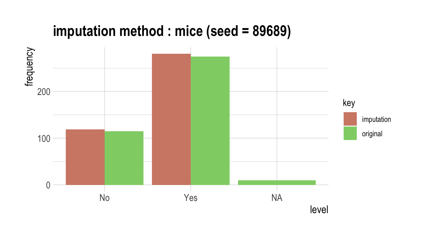
다음은 범주형 변수인 urban을 “mice” 방법으로 결측치를 대체한다. summary()는 결측치 대체 정보를 요약하고, plot()은 결측정보를 시각화한다.
library(mice)

urban <- imputate_na(carseats, Urban, US, method = "mice")
 iter imp variable
  1   1  Income  Urban
  1   2  Income  Urban
  1   3  Income  Urban
  1   4  Income  Urban
  1   5  Income  Urban
  2   1  Income  Urban
  2   2  Income  Urban
  2   3  Income  Urban
  2   4  Income  Urban
  2   5  Income  Urban
  3   1  Income  Urban
  3   2  Income  Urban
  3   3  Income  Urban
  3   4  Income  Urban
  3   5  Income  Urban
  4   1  Income  Urban
  4   2  Income  Urban
  4   3  Income  Urban
  4   4  Income  Urban
  4   5  Income  Urban
  5   1  Income  Urban
  5   2  Income  Urban
  5   3  Income  Urban
  5   4  Income  Urban
  5   5  Income  Urban
# result of imputate
urban
  [1] Yes Yes Yes Yes Yes No  Yes Yes No  No  No  Yes Yes Yes Yes No
 [17] Yes Yes No  Yes Yes No  Yes Yes Yes No  No  Yes Yes Yes Yes Yes
 [33] No  Yes Yes No  No  Yes Yes No  No  Yes Yes Yes Yes Yes No  Yes
 [49] Yes Yes Yes Yes Yes Yes No  Yes Yes Yes Yes Yes Yes No  Yes Yes
 [65] No  No  Yes Yes Yes Yes Yes No  Yes No  No  No  Yes No  Yes Yes
 [81] Yes Yes Yes Yes No  No  Yes No  Yes Yes No  Yes Yes Yes Yes Yes
 [97] No  Yes No  No  No  Yes No  Yes Yes Yes No  Yes Yes No  Yes Yes
[113] Yes Yes Yes Yes No  Yes Yes Yes Yes Yes Yes No  Yes No  Yes Yes
[129] Yes No  Yes Yes Yes Yes Yes No  No  Yes Yes No  Yes Yes Yes Yes
[145] No  Yes Yes No  No  Yes No  No  No  No  No  Yes Yes No  Yes No
[161] No  No  Yes No  No  Yes Yes Yes Yes Yes Yes Yes Yes Yes No  Yes
[177] No  Yes No  Yes Yes Yes Yes Yes No  Yes No  Yes Yes No  No  Yes
[193] No  Yes Yes Yes Yes Yes Yes Yes No  Yes No  Yes Yes Yes Yes No
[209] Yes No  No  Yes Yes Yes Yes Yes Yes No  Yes Yes Yes Yes Yes Yes
[225] No  Yes Yes Yes No  No  No  No  Yes No  No  Yes Yes Yes Yes Yes
[241] Yes Yes No  Yes Yes No  Yes Yes Yes Yes Yes No  Yes No  Yes Yes
[257] Yes Yes No  No  Yes Yes Yes Yes Yes Yes No  No  Yes Yes Yes Yes
[273] Yes Yes Yes Yes Yes Yes No  Yes No  No  No  No  No  Yes No  Yes
[289] No  Yes No  Yes Yes Yes Yes No  Yes Yes Yes No  Yes Yes Yes Yes
[305] Yes Yes Yes Yes Yes Yes Yes Yes Yes Yes Yes Yes Yes No  No  No
[321] Yes Yes Yes Yes Yes Yes Yes Yes Yes Yes No  Yes Yes Yes No  Yes
[337] Yes Yes Yes Yes Yes No  No  Yes No  Yes No  No  Yes No  No  No
[353] Yes No  Yes Yes Yes Yes Yes Yes No  No  Yes Yes Yes No  No  Yes
[369] No  Yes Yes Yes No  Yes Yes Yes Yes Yes Yes Yes Yes Yes Yes Yes
[385] Yes Yes Yes No  Yes Yes Yes Yes Yes No  Yes Yes No  Yes Yes Yes
attr(,"var_type")
[1] categorical
attr(,"method")
[1] mice
attr(,"na_pos")
 [1]  38  90 159 206 237 252 281 283 335 378
attr(,"seed")
[1] 89689
attr(,"type")
[1] missing values
attr(,"message")
[1] complete imputation
attr(,"success")
[1] TRUE
Levels: No Yes
# summary of imputate
summary(urban)
* Impute missing values based on Multivariate Imputation by Chained Equations
 - method : mice
 - random seed : 89689

* Information of Imputation (before vs after)
     original imputation original_percent imputation_percent
No        115        119            28.75              29.75
Yes       275        281            68.75              70.25
<NA>       10          0             2.50               0.00
# viz of imputate
plot(urban)
dplyr과의 협업
다음은 dplyr를 이용해서 이상치를 대체한 Income 변수를 US의 수준별로 산술평균을 구하는 예제다.
# The mean before and after the imputation of the Income variable
carseats %>%
  mutate(Income_imp = imputate_na(carseats, Income, US, method = "knn")) %>%
  group_by(US) %>%
  summarise(orig = mean(Income, na.rm = TRUE),
    imputation = mean(Income_imp))
# A tibble: 2 x 3
  US     orig imputation
  <fct> <dbl>      <dbl>
1 No     65.7       65.5
2 Yes    71.3       71.5
이상치의 대체
imputate_outlier()을 이용한 이상치의 대체
imputate_outlier()는 변수에 포함된 이상치를 대체한다. 이상치가 포함된 예측변수(predictor)는 수치형 변수만 지원하며, 다음과 같은 method를 지원한다.
- predictor가 수치형 변수일 경우
- “mean” : 산술평균으로 대체
- “median” : 중위수로 대체
- “mode” : 최빈수로 대체
- “capping” : 상위 이상치를 95/백분위수로 대체하고 하위 이상치를 5/백분위수로 대체
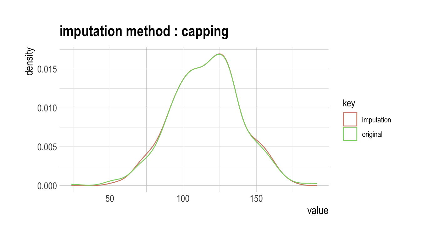
다음처럼 imputate_outlier()는 carseats의 수치형 변수인 Price를 “capping” 방법으로 이상치를 대체한다. summary()는 이상치 대체 정보를 요약하고, plot()은 결측정보를 시각화한다.
price <- imputate_outlier(carseats, Price, method = "capping")

# result of imputate
price
  [1] 120.00  83.00  80.00  97.00 128.00  72.00 108.00 120.00 124.00
 [10] 124.00 100.00  94.00 136.00  86.00 118.00 144.00 110.00 131.00
 [19]  68.00 121.00 131.00 109.00 138.00 109.00 113.00  82.00 131.00
 [28] 107.00  97.00 102.00  89.00 131.00 137.00 128.00 128.00  96.00
 [37] 100.00 110.00 102.00 138.00 126.00 124.00  77.00 134.00  95.00
 [46] 135.00  70.00 108.00  98.00 149.00 108.00 108.00 129.00 119.00
 [55] 144.00 154.00  84.00 117.00 103.00 114.00 123.00 107.00 133.00
 [64] 101.00 104.00 128.00  91.00 115.00 134.00  99.00  99.00 150.00
 [73] 116.00 104.00 136.00  92.00  70.00  89.00 145.00  90.00  79.00
 [82] 128.00 139.00  94.00 121.00 112.00 134.00 126.00 111.00 119.00
 [91] 103.00 107.00 125.00 104.00  84.00 148.00 132.00 129.00 127.00
[100] 107.00 106.00 118.00  97.00  96.00 138.00  97.00 139.00 108.00
[109] 103.00  90.00 116.00 151.00 125.00 127.00 106.00 129.00 128.00
[118] 119.00  99.00 128.00 131.00  87.00 108.00 155.00 120.00  77.00
[127] 133.00 116.00 126.00 147.00  77.00  94.00 136.00  97.00 131.00
[136] 120.00 120.00 118.00 109.00  94.00 129.00 131.00 104.00 159.00
[145] 123.00 117.00 131.00 119.00  97.00  87.00 114.00 103.00 128.00
[154] 150.00 110.00  69.00 157.00  90.00 112.00  70.00 111.00 160.00
[163] 149.00 106.00 141.00 155.05 137.00  93.00 117.00  77.00 118.00
[172]  55.00 110.00 128.00 155.05 122.00 154.00  94.00  81.00 116.00
[181] 149.00  91.00 140.00 102.00  97.00 107.00  86.00  96.00  90.00
[190] 104.00 101.00 173.00  93.00  96.00 128.00 112.00 133.00 138.00
[199] 128.00 126.00 146.00 134.00 130.00 157.00 124.00 132.00 160.00
[208]  97.00  64.00  90.00 123.00 120.00 105.00 139.00 107.00 144.00
[217] 144.00 111.00 120.00 116.00 124.00 107.00 145.00 125.00 141.00
[226]  82.00 122.00 101.00 163.00  72.00 114.00 122.00 105.00 120.00
[235] 129.00 132.00 108.00 135.00 133.00 118.00 121.00  94.00 135.00
[244] 110.00 100.00  88.00  90.00 151.00 101.00 117.00 156.00 132.00
[253] 117.00 122.00 129.00  81.00 144.00 112.00  81.00 100.00 101.00
[262] 118.00 132.00 115.00 159.00 129.00 112.00 112.00 105.00 166.00
[271]  89.00 110.00  63.00  86.00 119.00 132.00 130.00 125.00 151.00
[280] 158.00 145.00 105.00 154.00 117.00  96.00 131.00 113.00  72.00
[289]  97.00 156.00 103.00  89.00  74.00  89.00  99.00 137.00 123.00
[298] 104.00 130.00  96.00  99.00  87.00 110.00  99.00 134.00 132.00
[307] 133.00 120.00 126.00  80.00 166.00 132.00 135.00  54.00 129.00
[316] 171.00  72.00 136.00 130.00 129.00 152.00  98.00 139.00 103.00
[325] 150.00 104.00 122.00 104.00 111.00  89.00 112.00 134.00 104.00
[334] 147.00  83.00 110.00 143.00 102.00 101.00 126.00  91.00  93.00
[343] 118.00 121.00 126.00 149.00 125.00 112.00 107.00  96.00  91.00
[352] 105.00 122.00  92.00 145.00 146.00 164.00  72.00 118.00 130.00
[361] 114.00 104.00 110.00 108.00 131.00 162.00 134.00  77.00  79.00
[370] 122.00 119.00 126.00  98.00 116.00 118.00 124.00  92.00 125.00
[379] 119.00 107.00  89.00 151.00 121.00  68.00 112.00 132.00 160.00
[388] 115.00  78.00 107.00 111.00 124.00 130.00 120.00 139.00 128.00
[397] 120.00 159.00  95.00 120.00
attr(,"method")
[1] "capping"
attr(,"var_type")
[1] "numerical"
attr(,"outlier_pos")
[1]  43 126 166 175 368
attr(,"outliers")
[1]  24  49 191 185  53
attr(,"type")
[1] "outliers"
attr(,"message")
[1] "complete imputation"
attr(,"success")
[1] TRUE
attr(,"class")
[1] "imputation" "numeric"
# summary of imputate
summary(price)
Impute outliers with capping

* Information of Imputation (before vs after)
            Original  Imputation
n        400.0000000 400.0000000
na         0.0000000   0.0000000
mean     115.7950000 115.8927500
sd        23.6766644  22.6109187
se_mean    1.1838332   1.1305459
IQR       31.0000000  31.0000000
skewness  -0.1252862  -0.0461621
kurtosis   0.4518850  -0.3030578
p00       24.0000000  54.0000000
p01       54.9900000  67.9600000
p05       77.0000000  77.0000000
p10       87.0000000  87.0000000
p20       96.8000000  96.8000000
p25      100.0000000 100.0000000
p30      104.0000000 104.0000000
p40      110.0000000 110.0000000
p50      117.0000000 117.0000000
p60      122.0000000 122.0000000
p70      128.3000000 128.3000000
p75      131.0000000 131.0000000
p80      134.0000000 134.0000000
p90      146.0000000 146.0000000
p95      155.0500000 155.0025000
p99      166.0500000 164.0200000
p100     191.0000000 173.0000000
# viz of imputate
plot(price)
dplyr과의 협업
다음은 dplyr를 이용해서 이상치를 대체한 Price 변수를 US의 수준별로 산술평균을 구하는 예제다.
# The mean before and after the imputation of the Price variable
carseats %>%
  mutate(Price_imp = imputate_outlier(carseats, Price, method = "capping")) %>%
  group_by(US) %>%
  summarise(orig = mean(Price, na.rm = TRUE),
    imputation = mean(Price_imp, na.rm = TRUE))
# A tibble: 2 x 3
  US     orig imputation
  <fct> <dbl>      <dbl>
1 No     114.       114.
2 Yes    117.       117.
표준화와 치우친 데이터의 보정
transform()의 기능
transform()는 변수를 변환한다. 수치형 변수만 지원하며, 다음과 같은 method를 제공한다.
- 표준화
- “zscore” : z-score 변환. (x - mu) / sigma
- “minmax” : minmax 변환. (x - min) / (max - min)
- 치우침 보정
- “log” : log 변환. log(x)
- “log+1” : log 변환. log(x + 1). 0을 포함한 값들이 많을 때 유용함.
- “sqrt” : 제곱근 변환
- “1/x” : 1 / x 변환
- “x^2” : 제곱 변환
- “x^3” : 세제곱 변환
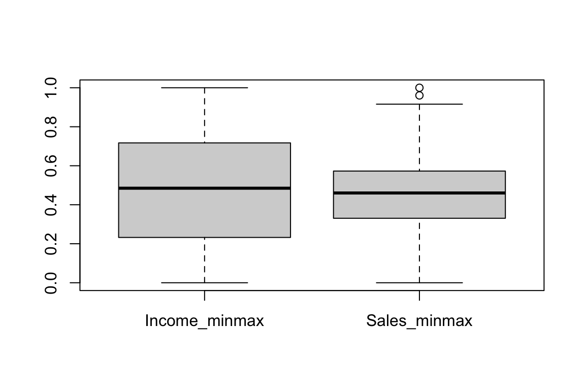
transform()을 이용한 표준화
표준화를 수행하는 method “zscore”와 “minmax”를 이용한다.
carseats %>%
  mutate(Income_minmax = transform(carseats$Income, method = "minmax"),
    Sales_minmax = transform(carseats$Sales, method = "minmax")) %>%
  select(Income_minmax, Sales_minmax) %>%
  boxplot()
transform()을 이용한 치우친 데이터의 보정
find_skewness()는 치우친 데이터를 찾기 위해서 왜도를 구한다.
# find index of skewed variables
find_skewness(carseats)
[1] 4# find names of skewed variables
find_skewness(carseats, index = FALSE)
[1] "Advertising"# compute the skewness
find_skewness(carseats, value = TRUE)
      Sales   CompPrice      Income Advertising  Population
      0.185      -0.043       0.036       0.637      -0.051
      Price         Age   Education
     -0.125      -0.077       0.044
# compute the skewness & filtering with threshold
find_skewness(carseats, value = TRUE, thres = 0.1)
      Sales Advertising       Price
0.185 0.637 -0.125 Advertising의 왜도가 0.637로 좌측으로 어느정도 기울어져 있어서 다음처럼 transformation()를 이용해서 “log” 방법으로 변환한다. summary()는 변환정보를 요약하고, plot()은 변환정보를 시각화한다.
Advertising_log = transform(carseats$Advertising, method = "log")

# result of transformation
head(Advertising_log)
[1] 2.397895 2.772589 2.302585 1.386294 1.098612 2.564949# summary of transformation
summary(Advertising_log)
* Resolving Skewness with log

* Information of Transformation (before vs after)
            Original Transformation
n        400.0000000    400.0000000
na         0.0000000      0.0000000
mean       6.6350000           -Inf
sd         6.6503642            NaN
se_mean    0.3325182            NaN
IQR       12.0000000            Inf
skewness   0.6395858            NaN
kurtosis  -0.5451178            NaN
p00        0.0000000           -Inf
p01        0.0000000           -Inf
p05        0.0000000           -Inf
p10        0.0000000           -Inf
p20        0.0000000           -Inf
p25        0.0000000           -Inf
p30        0.0000000           -Inf
p40        2.0000000      0.6931472
p50        5.0000000      1.6094379
p60        8.4000000      2.1265548
p70       11.0000000      2.3978953
p75       12.0000000      2.4849066
p80       13.0000000      2.5649494
p90       16.0000000      2.7725887
p95       19.0000000      2.9444390
p99       23.0100000      3.1359198
p100      29.0000000      3.3672958
# viz of transformation
plot(Advertising_log)
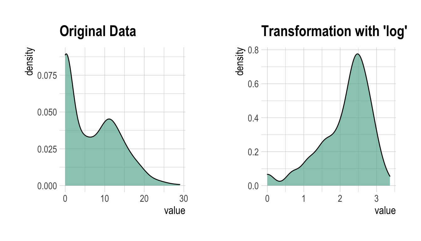
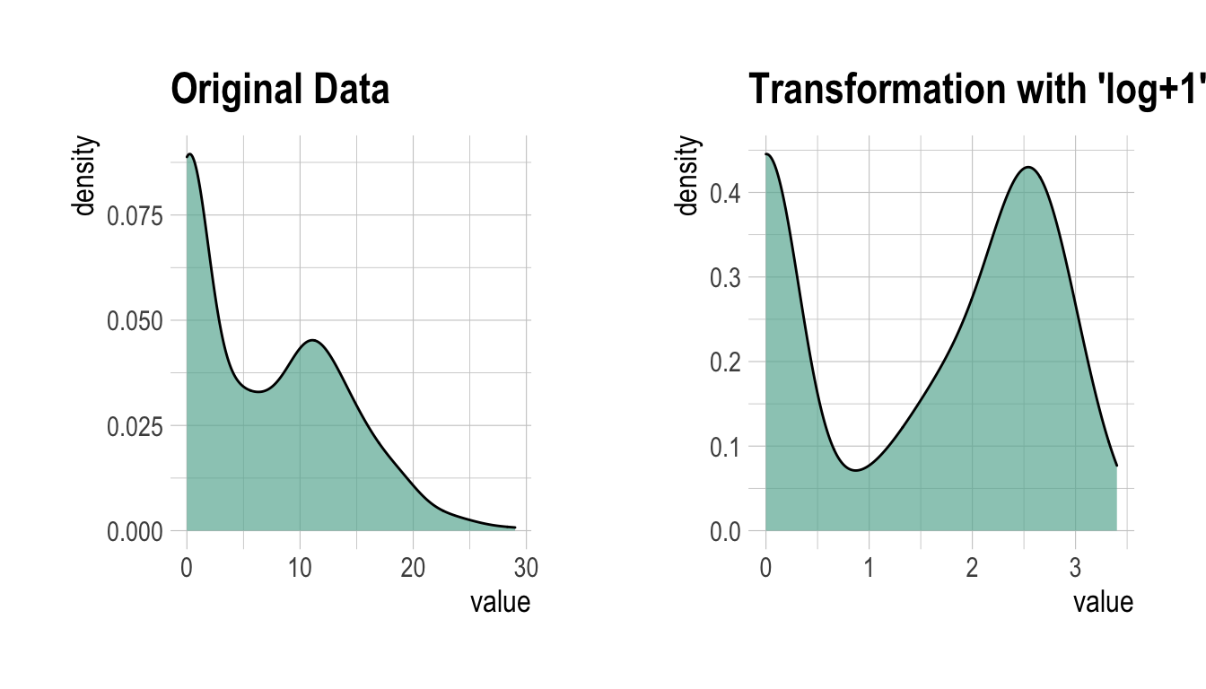
log 변환된 값에 -Inf가 포함되어 있는 것으로 보아 원 데이터에 0이 포함되어 있는 듯하다. 그래서 이번에는 “log+1” 방법으로 변환한다.
Advertising_log <- transform(carseats$Advertising, method = "log+1")

# result of transformation
head(Advertising_log)
[1] 2.484907 2.833213 2.397895 1.609438 1.386294 2.639057# summary of transformation
summary(Advertising_log)
* Resolving Skewness with log+1

* Information of Transformation (before vs after)
            Original Transformation
n        400.0000000   400.00000000
na         0.0000000     0.00000000
mean       6.6350000     1.46247709
sd         6.6503642     1.19436323
se_mean    0.3325182     0.05971816
IQR       12.0000000     2.56494936
skewness   0.6395858    -0.19852549
kurtosis  -0.5451178    -1.66342876
p00        0.0000000     0.00000000
p01        0.0000000     0.00000000
p05        0.0000000     0.00000000
p10        0.0000000     0.00000000
p20        0.0000000     0.00000000
p25        0.0000000     0.00000000
p30        0.0000000     0.00000000
p40        2.0000000     1.09861229
p50        5.0000000     1.79175947
p60        8.4000000     2.23936878
p70       11.0000000     2.48490665
p75       12.0000000     2.56494936
p80       13.0000000     2.63905733
p90       16.0000000     2.83321334
p95       19.0000000     2.99573227
p99       23.0100000     3.17846205
p100      29.0000000     3.40119738
# viz of transformation
plot(Advertising_log)
Binning
binning()을 이용한 개별 변수의 Binning
binning()는 수치형 변수를 비닝하여 범주형 변수로 변환한다. 다음과 같은 type의 비닝을 지원한다.
- “quantile” : 동일한 돗수가 포함되도록 quantile을 이용하여 범주화
- “equal” : 동일한 길이의 구간을 갖도록 범주화
- “pretty” : 적당히 보기 좋은 구간으로 범주화
- “kmeans” : K-means clustering 기법을 이용한 범주화
- “bclust” : Bagged clustering 기법을 이용한 범주화
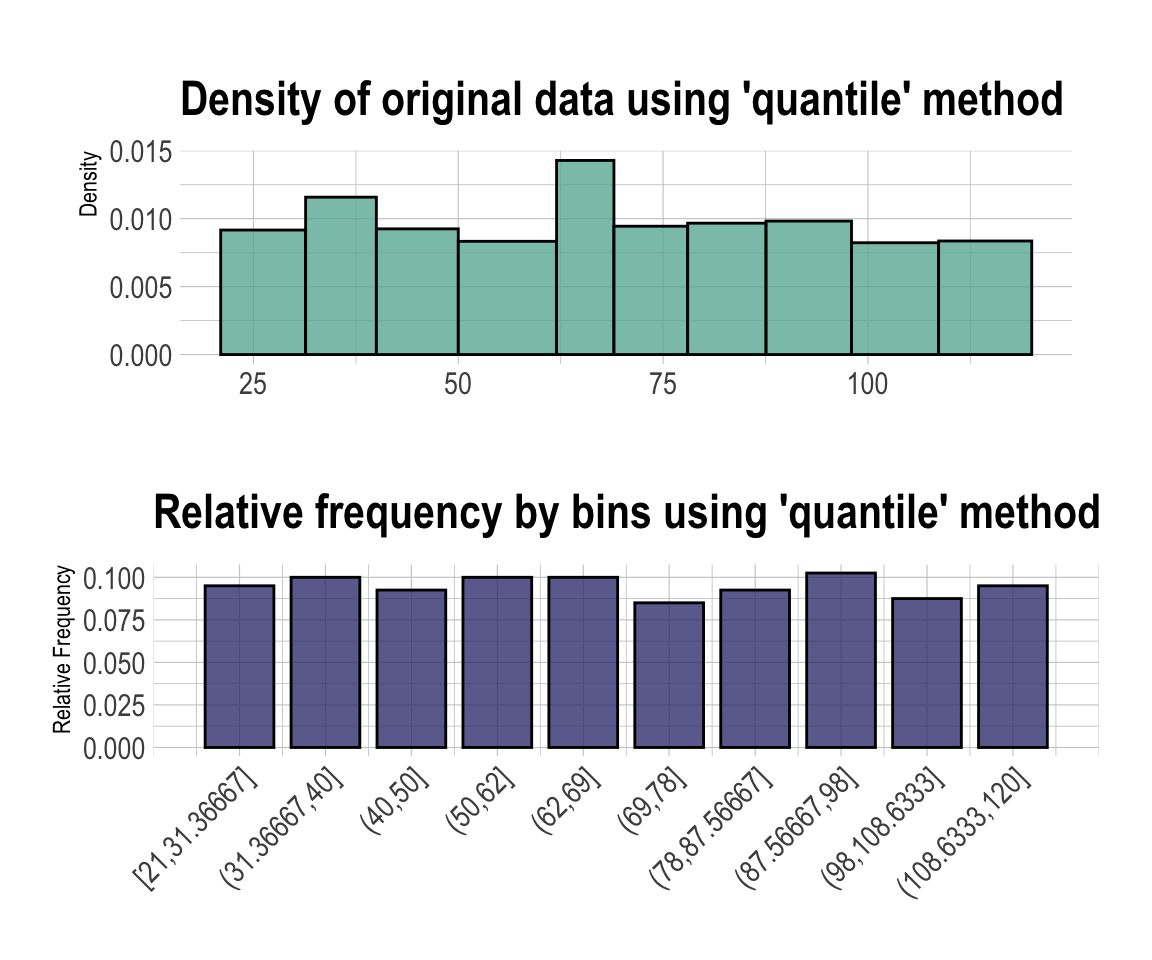
binning()을 이용하여 Income을 비닝하는 몇 가지의 방법을 예시한다.:
# Binning the carat variable. default type argument is "quantile"
bin <- binning(carseats$Income)
# Print bins class object
bin
binned type: quantile
number of bins: 10
x
 [21,31.36667]  (31.36667,40]        (40,50]        (50,62]
            38             40             37             40
       (62,69]        (69,78]  (78,87.56667]  (87.56667,98]
            40             34             37             41
 (98,108.6333] (108.6333,120]           <NA>
            35             38             20
# Summarise bins class object
summary(bin)
           levels freq   rate
1   [21,31.36667]   38 0.0950
2   (31.36667,40]   40 0.1000
3         (40,50]   37 0.0925
4         (50,62]   40 0.1000
5         (62,69]   40 0.1000
6         (69,78]   34 0.0850
7   (78,87.56667]   37 0.0925
8   (87.56667,98]   41 0.1025
9   (98,108.6333]   35 0.0875
10 (108.6333,120]   38 0.0950
11           <NA>   20 0.0500
# Plot bins class object
plot(bin)
# Using labels argument
bin <- binning(carseats$Income, nbins = 4,
              labels = c("LQ1", "UQ1", "LQ3", "UQ3"))
bin
binned type: quantile
number of bins: 4
x
 LQ1  UQ1  LQ3  UQ3 <NA>
  98   97   91   94   20
# Using another type argument
binning(carseats$Income, nbins = 5, type = "equal")
binned type: equal
number of bins: 5
x
   [21,40.8]  (40.8,60.6]  (60.6,80.4] (80.4,100.2]  (100.2,120]
          78           68           92           79           63
        <NA>
20 binning(carseats$Income, nbins = 5, type = "pretty")
binned type: pretty
number of bins: 5
x
  [20,40]   (40,60]   (60,80]  (80,100] (100,120]      <NA>
78 68 92 79 63 20 binning(carseats$Income, nbins = 5, type = "kmeans")
binned type: kmeans
number of bins: 5
x
     [21,49]    (49,70.5]  (70.5,87.5] (87.5,104.5]  (104.5,120]
         113           86           67           63           51
        <NA>
20 binning(carseats$Income, nbins = 5, type = "bclust")
binned type: bclust
number of bins: 5
x
  [21,50.5] (50.5,65.5]   (65.5,85]  (85,108.5] (108.5,120]
        115          55          91          81          38
       <NA>
         20
# -------------------------
# Using pipes & dplyr
# -------------------------
library(dplyr)
carseats %>%
mutate(Income_bin = binning(carseats$Income)) %>%
group_by(ShelveLoc, Income_bin) %>%
summarise(freq = n()) %>%
arrange(desc(freq)) %>%
head(10)
# A tibble: 10 x 3
# Groups:   ShelveLoc [1]
   ShelveLoc Income_bin      freq
   <fct>     <ord>          <int>
 1 Medium    [21,31.36667]     25
 2 Medium    (62,69]           23
 3 Medium    (50,62]           22
 4 Medium    (31.36667,40]     21
 5 Medium    (40,50]           20
 6 Medium    (69,78]           20
 7 Medium    (108.6333,120]    20
 8 Medium    (78,87.56667]     19
 9 Medium    (87.56667,98]     19
10 Medium (98,108.6333] 19binning_by()을 이용한 Optimal Binning
binning_by()는 수치형 변수를 Optimal Binning하여 범주형 변수로 변환한다. 이 방법은 스코어카드 모형을 개발할때 자주 사용하는 방법이다.
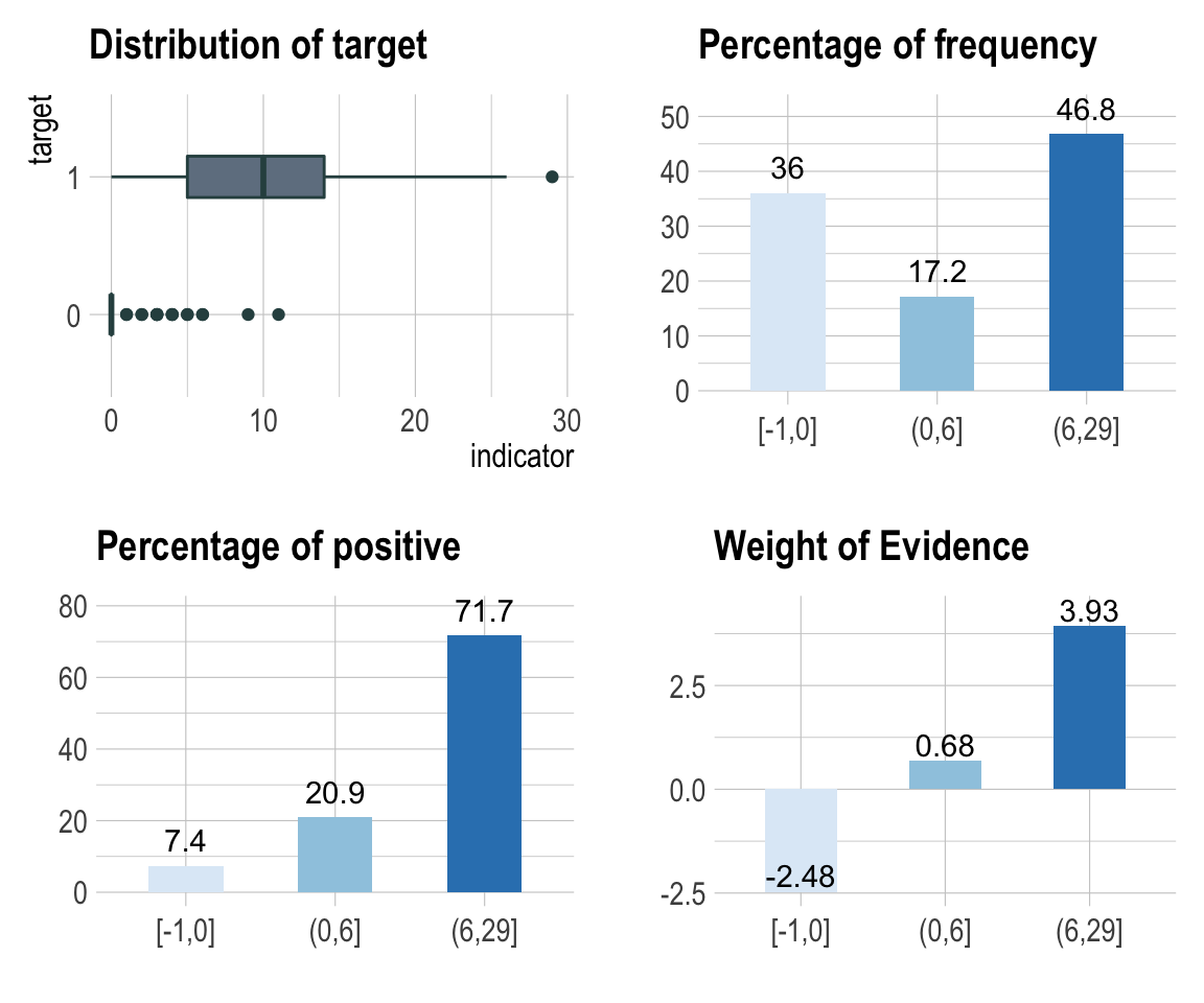
다음의 binning_by() 예제는 US가 binary class를 갖는 target 변수일 경우에 Advertising를 Optimal Binning하는 방법의 예시다.
# optimal binning
bin <- binning_by(carseats, "US", "Advertising")
` US ` ~ ` Advertising `
<environment: 0x7fd84661f238>
bin
binned type: optimal
number of bins: 3
x
[-1,0]  (0,6] (6,29]
   144     69    187
# summary optimal_bins class
summary(bin)
── Binning Table ──────────────────────── Several Metrics ──
     Bin CntRec CntPos CntNeg RatePos RateNeg    Odds      WoE
1 [-1,0]    144     19    125 0.07364 0.88028  0.1520 -2.48101
2  (0,6]     69     54     15 0.20930 0.10563  3.6000  0.68380
3 (6,29]    187    185      2 0.71705 0.01408 92.5000  3.93008
4  Total    400    258    142 1.00000 1.00000  1.8169       NA
       IV     JSD     AUC
1 2.00128 0.20093 0.03241
2 0.07089 0.00869 0.01883
3 2.76272 0.21861 0.00903
4 4.83489 0.42823 0.06028

── General Metrics ─────────────────────────────────────────
• Gini index                       :  -0.87944
• IV (Jeffrey)                     :  4.83489
• JS (Jensen-Shannon) Divergence   :  0.42823
• Kolmogorov-Smirnov Statistics    :  0.80664
• HHI (Herfindahl-Hirschman Index) :  0.37791
• HHI (normalized)                 :  0.06687
• Cramer's V                       :  0.81863

── Significance Tests ──────────────────── Chisquare Test ──
   Bin A  Bin B statistics      p_value
1 [-1,0]  (0,6]   87.67064 7.731349e-21
2  (0,6] (6,29]   34.73349 3.780706e-09
# information value
attr(bin, "iv")
NULL# information value table
attr(bin, "ivtable")
NULL# visualize optimal_bins class
plot(bin, sub = "bins of Advertising variable")
보고서 생성
diagnose_report()를 이용한 진단 보고서 작성
diagnose_report()는 데이터 프레임이나 데이터 프레임을 상속받은 객체(tbl_df, tbl 등)의 모든 변수들에 대해서 데이터 진단을 수행한다.
diagnose_report()는 진단 보고서를 다음과 같은 두 개의 형태로 작성한다.
- Latex에 기반한 pdf 파일
- html 파일
보고서의 목차는 다음과 같다.
- 데이터 진단
- 데이터 품질 총괄
- 전체변수 품질현황 목록
- 결측치 진단
- 유일값 진단(문자형과 범주형)
- 유일값 진단(수치형)
- 데이터 품질 상세
- 범주형 변수 품질 현황
- 수치형 변수 품질 현황
- 수치변수 품질현황 (zero)
- 수치변수 품질현황 (minus)
- 데이터 품질 총괄
- 이상치 진단
- 데이터 품질 총괄
- 수치변수의 이상치 진단
- 이상치 상세 진단
- 데이터 품질 총괄
다음은 tbl_df 클래스 객체인 flights의 품질진단 리포트를 작성한다. 파일 형식은 pdf이며, 파일이름은 DataDiagnosis_Report.pdf다.
flights %>%
  diagnose_report()
다음은 DataDiagnosis_Report.html라는 이름의 html 형식의 보고서를 생성한다.
flights %>%
  diagnose_report(output_format = "html")
다음은 Diagn.html라는 이름의 html 형식의 보고서를 생성한다.
flights %>%
  diagnose_report(output_format = "html", output_file = "Diagn.html")
데이터 진단 보고서는 데이터 진단 과정에 도움을 주기 위한 자동화 보고서다. 보고서 결과를 참고하여 데이터 보완이나 재획득을 판단한다.
eda_report()를 이용한 EDA 보고서 작성
eda_report()는 데이터 프레임이나 데이터 프레임을 상속받은 객체(tbl_df, tbl 등)의 모든 변수들에 대해서 EDA를 수행한다.
eda_report()는 EDA 보고서를 다음과 같은 두 개의 형태로 작성한다.
- Latex에 기반한 pdf 파일
- html 파일
보고서의 목차는 다음과 같다.
- 개요
- 데이터셋 정보
- 변수 정보
- 수치변수
- 일변량 변수 EDA
- 기술통계
- 수치변수의 정규성 검정
- 통계량과 시각화 정보
- 변수들간의 관계
- 상관계수
- 변수 조합의 상관계수
- 수치변수의 상관행렬 플롯
- 상관계수
- Target 변수 기반의 EDA
- 그룹화된 기술통계
- 그룹화된 Target과 수치형 변수 관계
- 그룹화된 Target과 범주형 변수 관계
- 그룹화된 Target과 변수들간의 관계
- 그룹화된 Target과 수치형 변수의 상관계수
- 그룹화된 Target과 수치형 변수의 상관행렬 플롯
- 그룹화된 기술통계
다음은 carseats의 품질진단 리포트를 작성한다. 파일 형식은 pdf이며, 파일이름은 EDA_Report.pdf다.
carseats %>%
  eda_report(target = Sales)
다음은 EDA.html라는 이름의 html 형식의 보고서를 생성한다.
carseats %>%
  eda_report(target = Sales, output_format = "html", output_file = "EDA.html")
EDA 보고서는 EDA 과정에 도움을 주기 위한 자동화 보고서다. 보고서 결과를 참고하여 데이터 분석 시나리오를 설계한다.
transformation_report()를 이용한 데이터변환 보고서 작성
transformation_report()는 데이터 프레임이나 데이터 프레임을 상속받은 객체(tbl_df, tbl 등)의 모든 변수들에 대해서 데이터변환 보고서를 작성한다.
transformation_report()는 데이터변환 보고서를 다음과 같은 두 개의 형태로 작성한다.
- Latex에 기반한 pdf 파일
- html 파일
보고서의 목차는 다음과 같다.:
- 값의 대체
- 결측치
- 결측치의 대체 정보
- (해당 변수들)
- 이상치
- 이상치의 대체 정보
- (해당 변수들)
- 결측치
- 치우침의 해결
- 치우친 변수들의 정보
- (해당 변수들)
- 치우친 변수들의 정보
- 비닝
- 비닝을 위한 수치형 변수들
- 비닝
- (해당 변수들)
- Optimal 비닝
- (해당 변수들)
다음은 carseats의 데이터변환 보고서를 작성한다. 파일 형식은 pdf이며, 파일이름은 Transformation_Report.pdf다.
carseats %>%
  transformation_report(target = US)
다음은 transformation.html라는 이름의 html 형식의 보고서를 생성한다.
carseats %>%
  transformation_report(target = US, output_format = "html",
    output_file = "transformation.html")
데이터변환 보고서는 데이터 변환 과정에 도움을 주기 위한 자동화 보고서다. 보고서 결과를 참고하여 데이터 변환 시나리오를 설계한다.
데이터변환 리포트 내용
pdf 파일의 내용
보고서의 표지
보고서의 표지는 다음 그림과 같다.:
(#fig:eda_title_pdf)EDA report cover
보고서 차례
보고서의 차례는 다음 그림과 같다.:
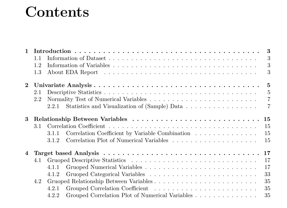
Figure 1: EDA Report Contents
표의 표현
대부분의 정보는 보고서에 표로 표시된다. 다음 예제는 표의 예를 보여준다.:
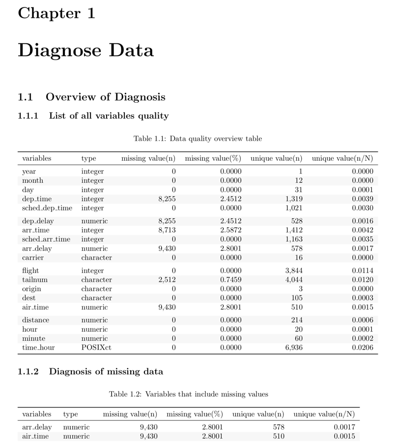
Figure 2: Sample data diagnostic report table
시각화의 표현
EDA 보고서에서는 선형 관계에 대한 정보를 표와 시각화 결과로 표현한다. 결과는 다음 그림과 같다.:
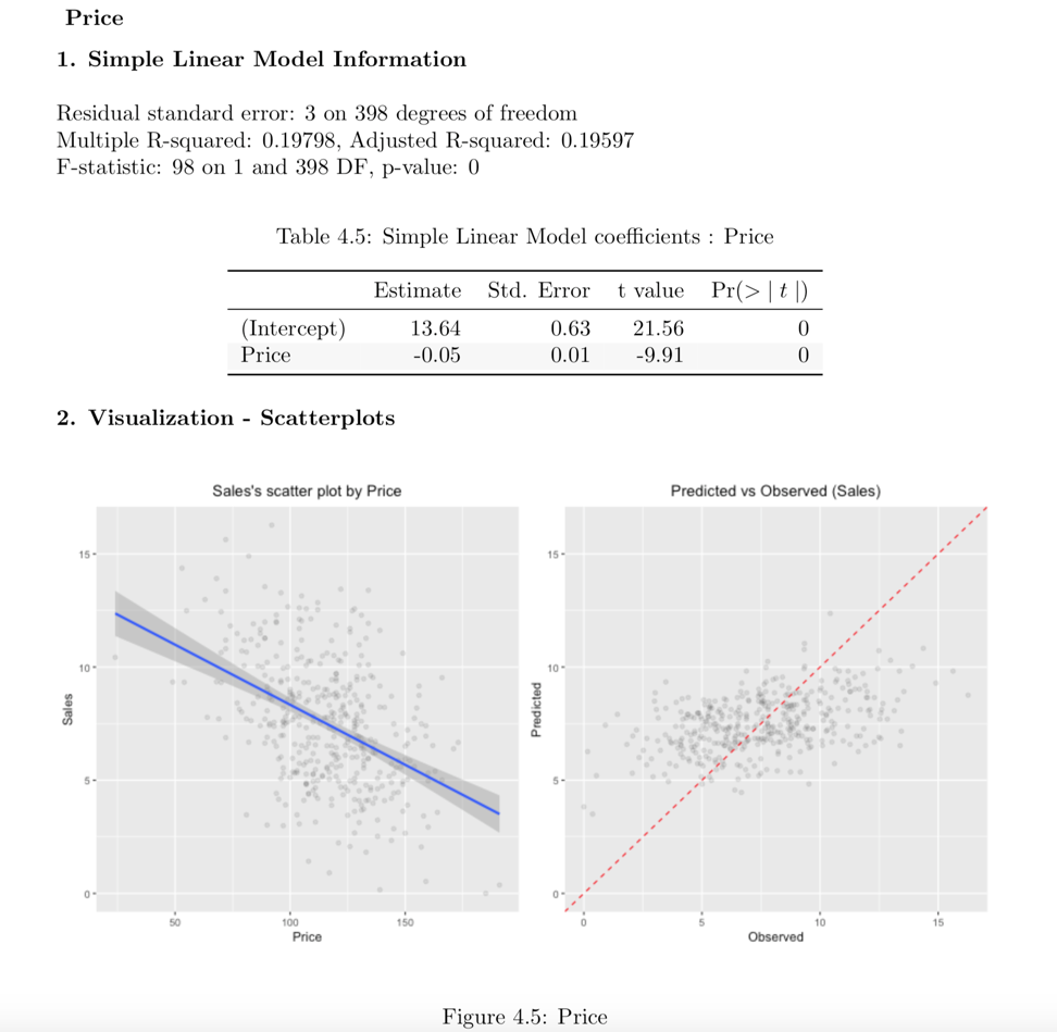
Figure 3: Linear relationship information in EDA reports
html 파일의 내용
보고서의 표지 및 차례
보고서의 표지와 차례는 다음 그림과 같다.::

Figure 4: EDA report titles and table of contents
표의 표현
많은 정보가 보고서에서 표로 표현된다. 다음 그림은 html 파일에서의 표의 예시다.:
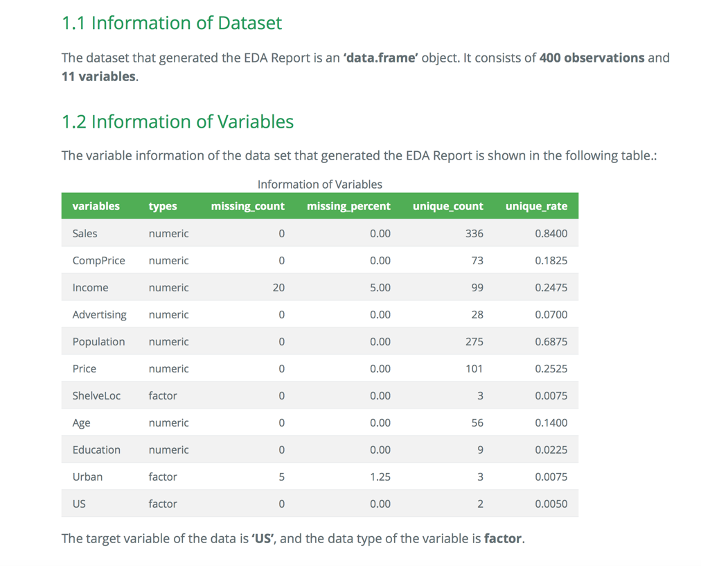
Figure 5: EDA report table example (Web)
시각화의 표현
EDA 보고서에서 정규성 검정 정보는 시각화 결과를 포함한다. html 파일에서의 결과는 다음 그림과 같다.:
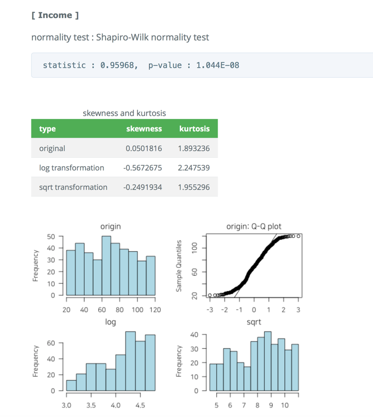
Figure 6: EDA Report Normality Test Information (Web)