The binning_rgr() finding intervals for numerical variable using recursive information gain ratio maximization.
binning_rgr(.data, y, x, min_perc_bins = 0.1, max_n_bins = 5, ordered = TRUE)Arguments
- .data
a data frame.
- y
character. name of binary response variable. The variable must character of factor.
- x
character. name of continuous characteristic variable. At least 5 different values. and Inf is not allowed.
- min_perc_bins
numeric. minimum percetange of rows for each split or segment (controls the sample size), 0.1 (or 10 percent) as default.
- max_n_bins
integer. maximum number of bins or segments to split the input variable, 5 bins as default.
- ordered
logical. whether to build an ordered factor or not.
Value
an object of "infogain_bins" class. Attributes of "infogain_bins" class is as follows.
class : "infogain_bins".
type : binning type, "infogain".
breaks : numeric. the number of intervals into which x is to be cut.
levels : character. levels of binned value.
raw : numeric. raw data, x argument value.
target : integer. binary response variable.
x_var : character. name of x variable.
y_var : character. name of y variable.
Details
This function can be usefully used when developing a model that predicts y.
See also
Examples
# \donttest{
library(dplyr)
# binning by recursive information gain ratio maximization using character
bin <- binning_rgr(heartfailure, "death_event", "creatinine")
# binning by recursive information gain ratio maximization using name
bin <- binning_rgr(heartfailure, death_event, creatinine)
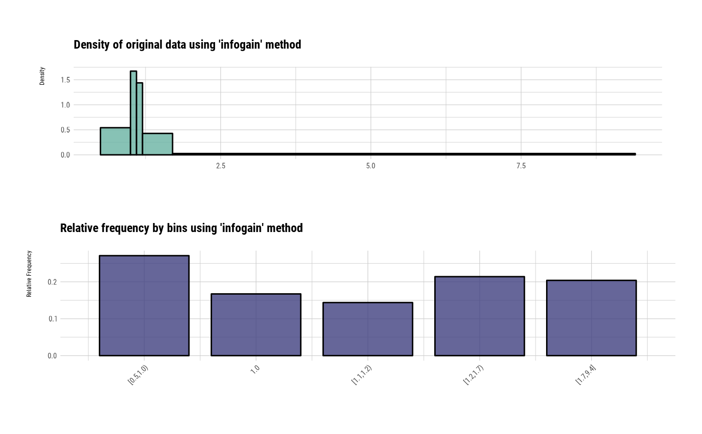
bin
#> binned type: infogain
#> number of bins: 5
#> x
#> [0.5,1.0) 1.0 [1.1,1.2) [1.2,1.7) [1.7,9.4]
#> 81 50 43 64 61
# summary optimal_bins class
summary(bin)
#> levels freq rate
#> 1 [0.5,1.0) 81 0.2709030
#> 2 1.0 50 0.1672241
#> 3 [1.1,1.2) 43 0.1438127
#> 4 [1.2,1.7) 64 0.2140468
#> 5 [1.7,9.4] 61 0.2040134
# visualize all information for optimal_bins class
plot(bin)
#> Don't know how to automatically pick scale for object of type <table>.
#> Defaulting to continuous.
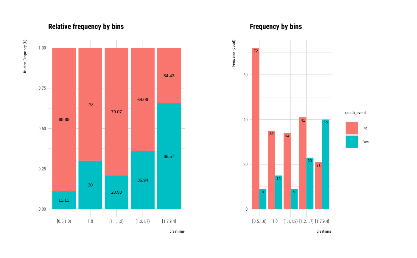
 # visualize WoE information for optimal_bins class
plot(bin, type = "cross")
# visualize WoE information for optimal_bins class
plot(bin, type = "cross")
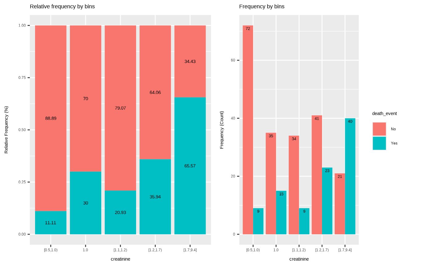
 # visualize all information without typographic
plot(bin, type = "cross", typographic = FALSE)
# visualize all information without typographic
plot(bin, type = "cross", typographic = FALSE)
 # extract binned results
extract(bin) %>%
head(20)
#> [1] [1.7,9.4] [1.1,1.2) [1.2,1.7) [1.7,9.4] [1.7,9.4] [1.7,9.4] [1.2,1.7)
#> [8] [1.1,1.2) [1.2,1.7) [1.7,9.4] [1.7,9.4] [0.5,1.0) [1.1,1.2) [1.1,1.2)
#> [15] 1.0 [1.2,1.7) [0.5,1.0) [0.5,1.0) 1.0 [1.7,9.4]
#> Levels: [0.5,1.0) < 1.0 < [1.1,1.2) < [1.2,1.7) < [1.7,9.4]
# }
# extract binned results
extract(bin) %>%
head(20)
#> [1] [1.7,9.4] [1.1,1.2) [1.2,1.7) [1.7,9.4] [1.7,9.4] [1.7,9.4] [1.2,1.7)
#> [8] [1.1,1.2) [1.2,1.7) [1.7,9.4] [1.7,9.4] [0.5,1.0) [1.1,1.2) [1.1,1.2)
#> [15] 1.0 [1.2,1.7) [0.5,1.0) [0.5,1.0) 1.0 [1.7,9.4]
#> Levels: [0.5,1.0) < 1.0 < [1.1,1.2) < [1.2,1.7) < [1.7,9.4]
# }