The compare_numeric() compute information to examine the relationship between numerical variables.
compare_numeric(.data, ...)

# S3 method for class 'data.frame'
compare_numeric(.data, ...)
Arguments
- .data
a data.frame or a
tbl_df.- ...
one or more unquoted expressions separated by commas. You can treat variable names like they are positions. Positive values select variables; negative values to drop variables. These arguments are automatically quoted and evaluated in a context where column names represent column positions. They support unquoting and splicing.
Value
An object of the class as compare based list. The information to examine the relationship between numerical variables is as follows each components. - correlation component : Pearson's correlation coefficient.
var1 : factor. The level of the first variable to compare. 'var1' is the name of the first variable to be compared.
var2 : factor. The level of the second variable to compare. 'var2' is the name of the second variable to be compared.
coef_corr : double. Pearson's correlation coefficient.
- linear component : linear model summaries
var1 : factor. The level of the first variable to compare. 'var1' is the name of the first variable to be compared.
var2 : factor.The level of the second variable to compare. 'var2' is the name of the second variable to be compared.
r.squared : double. The percent of variance explained by the model.
adj.r.squared : double. r.squared adjusted based on the degrees of freedom.
sigma : double. The square root of the estimated residual variance.
statistic : double. F-statistic.
p.value : double. p-value from the F test, describing whether the full regression is significant.
df : integer degrees of freedom.
logLik : double. the log-likelihood of data under the model.
AIC : double. the Akaike Information Criterion.
BIC : double. the Bayesian Information Criterion.
deviance : double. deviance.
df.residual : integer residual degrees of freedom.
Details
It is important to understand the relationship between numerical variables in EDA. compare_numeric() compares relations by pair combination of all numerical variables. and return compare_numeric class that based list object.
Attributes of return object
Attributes of compare_numeric class is as follows.
raw : a data.frame or a
tbl_df. Data containing variables to be compared. Save it for visualization with plot.compare_numeric().variables : character. List of variables selected for comparison.
combination : matrix. It consists of pairs of variables to compare.
Examples
# \donttest{
# Generate data for the example
heartfailure2 <- heartfailure[, c("platelets", "creatinine", "sodium")]
library(dplyr)
# Compare the all numerical variables
all_var <- compare_numeric(heartfailure2)
# Print compare_numeric class object
all_var
#> $correlation
#> # A tibble: 3 × 3
#> var1 var2 coef_corr
#> <chr> <chr> <dbl>
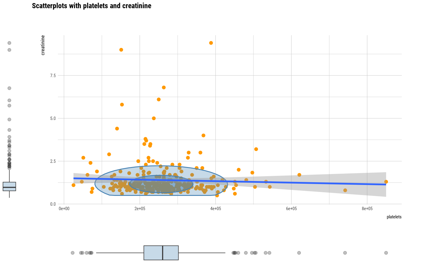
#> 1 platelets creatinine -0.0412
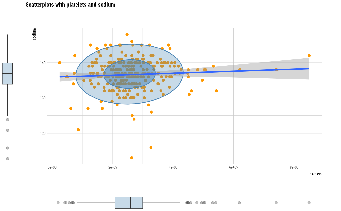
#> 2 platelets sodium 0.0621
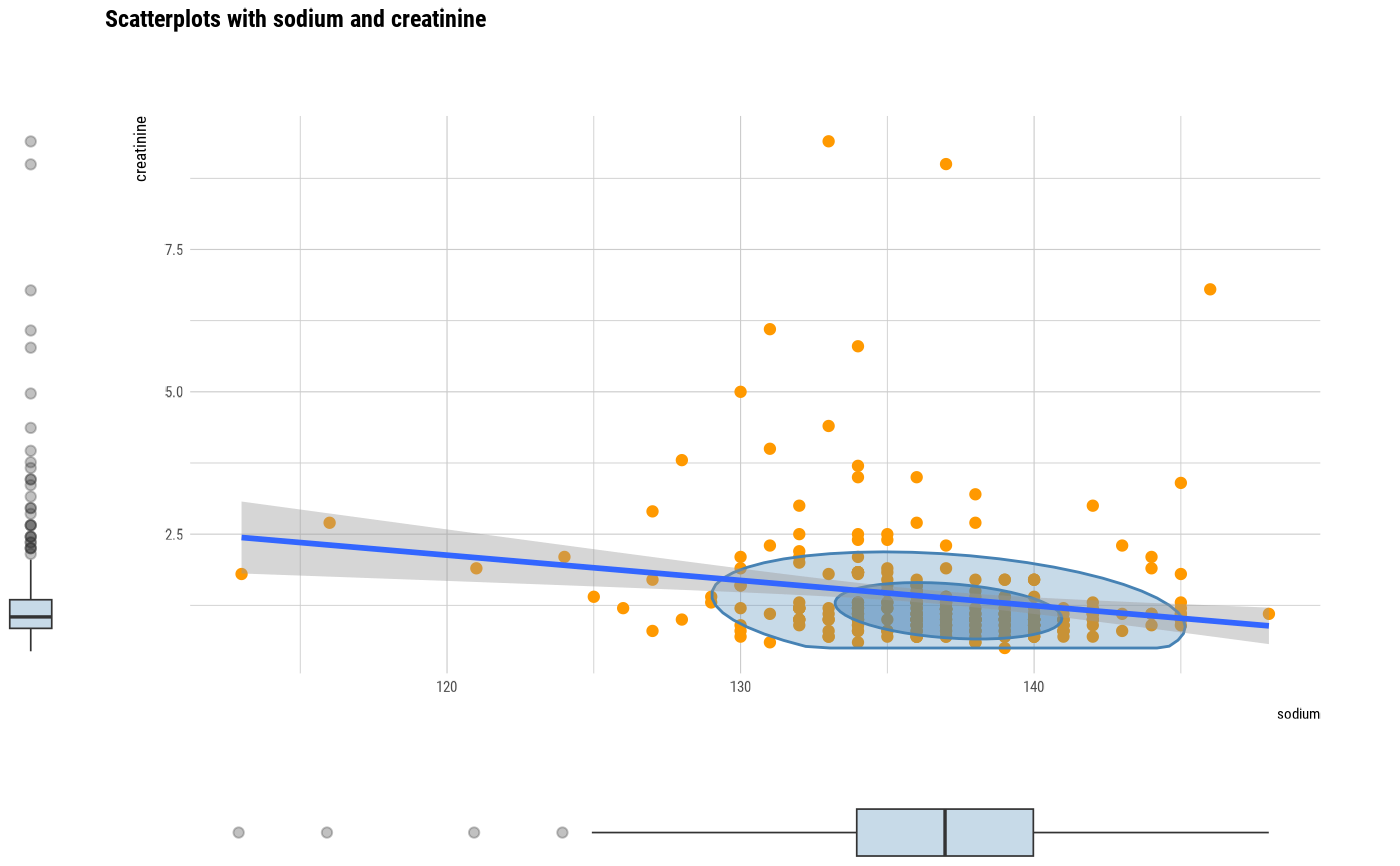
#> 3 creatinine sodium -0.189
#>
#> $linear
#> # A tibble: 3 × 14
#> var1 var2 r.squared adj.r.squared sigma statistic p.value df logLik
#> <chr> <chr> <dbl> <dbl> <dbl> <dbl> <dbl> <dbl> <dbl>
#> 1 platelets crea… 0.00170 -0.00166 9.79e4 0.505 0.478 1 -3859.
#> 2 platelets sodi… 0.00386 0.000505 9.78e4 1.15 0.284 1 -3859.
#> 3 creatinine sodi… 0.0358 0.0325 1.02e0 11.0 0.00102 1 -428.
#> # ℹ 5 more variables: AIC <dbl>, BIC <dbl>, deviance <dbl>, df.residual <int>,
#> # nobs <int>
#>
# Compare the correlation that case of joint the sodium variable
all_var %>%
"$"(correlation) %>%
filter(var1 == "sodium" | var2 == "sodium") %>%
arrange(desc(abs(coef_corr)))
#> # A tibble: 2 × 3
#> var1 var2 coef_corr
#> <chr> <chr> <dbl>
#> 1 creatinine sodium -0.189
#> 2 platelets sodium 0.0621
# Compare the correlation that case of abs(coef_corr) > 0.1
all_var %>%
"$"(correlation) %>%
filter(abs(coef_corr) > 0.1)
#> # A tibble: 1 × 3
#> var1 var2 coef_corr
#> <chr> <chr> <dbl>
#> 1 creatinine sodium -0.189
# Compare the linear model that case of joint the sodium variable
all_var %>%
"$"(linear) %>%
filter(var1 == "sodium" | var2 == "sodium") %>%
arrange(desc(r.squared))
#> # A tibble: 2 × 14
#> var1 var2 r.squared adj.r.squared sigma statistic p.value df logLik
#> <chr> <chr> <dbl> <dbl> <dbl> <dbl> <dbl> <dbl> <dbl>
#> 1 creatinine sodi… 0.0358 0.0325 1.02e0 11.0 0.00102 1 -428.
#> 2 platelets sodi… 0.00386 0.000505 9.78e4 1.15 0.284 1 -3859.
#> # ℹ 5 more variables: AIC <dbl>, BIC <dbl>, deviance <dbl>, df.residual <int>,
#> # nobs <int>
# Compare the two numerical variables
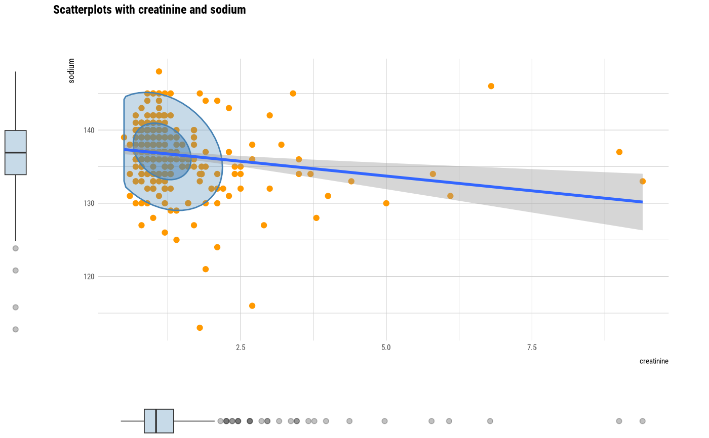
two_var <- compare_numeric(heartfailure2, sodium, creatinine)
# Print compare_numeric class objects
two_var
#> $correlation
#> # A tibble: 1 × 3
#> var1 var2 coef_corr
#> <chr> <chr> <dbl>
#> 1 sodium creatinine -0.189
#>
#> $linear
#> # A tibble: 1 × 14
#> var1 var2 r.squared adj.r.squared sigma statistic p.value df logLik AIC
#> <chr> <chr> <dbl> <dbl> <dbl> <dbl> <dbl> <dbl> <dbl> <dbl>
#> 1 sodi… crea… 0.0358 0.0325 4.34 11.0 0.00102 1 -862. 1730.
#> # ℹ 4 more variables: BIC <dbl>, deviance <dbl>, df.residual <int>, nobs <int>
#>
# Summary the all case : Return a invisible copy of an object.
stat <- summary(all_var)
#> ── Correlation check : abs(r) > 0.3 ───────────── Number of pairs is 0/3 ──
#> # A tibble: 0 × 3
#> # ℹ 3 variables: var1 <chr>, var2 <chr>, coef_corr <dbl>
#> ── R.squared check : R^2 > 0.1 ────────────────── Number of pairs is 0/3 ──
#> # A tibble: 0 × 14
#> # ℹ 14 variables: var1 <chr>, var2 <chr>, r.squared <dbl>, adj.r.squared <dbl>,
#> # sigma <dbl>, statistic <dbl>, p.value <dbl>, df <dbl>, logLik <dbl>,
#> # AIC <dbl>, BIC <dbl>, deviance <dbl>, df.residual <int>, nobs <int>
# Just correlation
summary(all_var, method = "correlation")
#> ── Correlation check : abs(r) > 0.3 ───────────── Number of pairs is 0/3 ──
#> # A tibble: 0 × 3
#> # ℹ 3 variables: var1 <chr>, var2 <chr>, coef_corr <dbl>
# Just correlation condition by r > 0.1
summary(all_var, method = "correlation", thres_corr = 0.1)
#> ── Correlation check : abs(r) > 0.1 ───────────── Number of pairs is 1/3 ──
#> # A tibble: 1 × 3
#> var1 var2 coef_corr
#> <chr> <chr> <dbl>
#> 1 creatinine sodium -0.189
# linear model summaries condition by R^2 > 0.05
summary(all_var, thres_rs = 0.05)
#> ── Correlation check : abs(r) > 0.3 ───────────── Number of pairs is 0/3 ──
#> # A tibble: 0 × 3
#> # ℹ 3 variables: var1 <chr>, var2 <chr>, coef_corr <dbl>
#> ── R.squared check : R^2 > 0.05 ───────────────── Number of pairs is 0/3 ──
#> # A tibble: 0 × 14
#> # ℹ 14 variables: var1 <chr>, var2 <chr>, r.squared <dbl>, adj.r.squared <dbl>,
#> # sigma <dbl>, statistic <dbl>, p.value <dbl>, df <dbl>, logLik <dbl>,
#> # AIC <dbl>, BIC <dbl>, deviance <dbl>, df.residual <int>, nobs <int>
# verbose is FALSE
summary(all_var, verbose = FALSE)
#> $correlation
#> # A tibble: 0 × 3
#> # ℹ 3 variables: var1 <chr>, var2 <chr>, coef_corr <dbl>
#>
#> $linear
#> # A tibble: 0 × 14
#> # ℹ 14 variables: var1 <chr>, var2 <chr>, r.squared <dbl>, adj.r.squared <dbl>,
#> # sigma <dbl>, statistic <dbl>, p.value <dbl>, df <dbl>, logLik <dbl>,
#> # AIC <dbl>, BIC <dbl>, deviance <dbl>, df.residual <int>, nobs <int>
#>
# plot all pair of variables
plot(all_var)
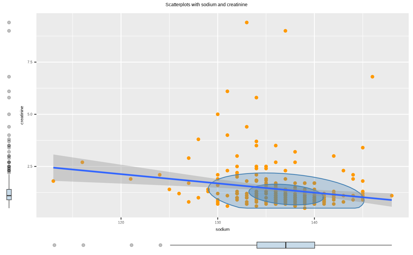
 # plot a pair of variables
plot(two_var)
# plot a pair of variables
plot(two_var)
 # plot all pair of variables by prompt
plot(all_var, prompt = TRUE)
# plot all pair of variables by prompt
plot(all_var, prompt = TRUE)


 # plot a pair of variables not focuses on typographic elements
plot(two_var, typographic = FALSE)
# plot a pair of variables not focuses on typographic elements
plot(two_var, typographic = FALSE)
 # }
# }