Diagnose Performance Binned Variable

The performance_bin() calculates metrics to evaluate the performance of binned variable for binomial classification model.

performance_bin(y, x, na.rm = FALSE)

Arguments

y: character or numeric, integer, factor. a binary response variable (0, 1). The variable must contain only the integers 0 and 1 as element. However, in the case of factor/character having two levels, it is performed while type conversion is performed in the calculation process.
x: integer or factor, character. At least 2 different values. and Inf is not allowed.
na.rm: logical. a logical indicating whether missing values should be removed.

Value

an object of "performance_bin" class. vaue of data.frame is as follows.

Bin : character. bins.
CntRec : integer. frequency by bins.
CntPos : integer. frequency of positive by bins.
CntNeg : integer. frequency of negative by bins.
CntCumPos : integer. cumulate frequency of positive by bins.
CntCumNeg : integer. cumulate frequency of negative by bins.
RatePos : integer. relative frequency of positive by bins.
RateNeg : integer. relative frequency of negative by bins.
RateCumPos : numeric. cumulate relative frequency of positive by bins.
RateCumNeg : numeric. cumulate relative frequency of negative by bins.
Odds : numeric. odd ratio.
LnOdds : numeric. loged odd ratio.
WoE : numeric. weight of evidence.
IV : numeric. Jeffrey's Information Value.
JSD : numeric. Jensen-Shannon Divergence.
AUC : numeric. AUC. area under curve.

Attributes of "performance_bin" class is as follows.

names : character. variable name of data.frame with "Binning Table".
class : character. name of class. "performance_bin" "data.frame".
row.names : character. row name of data.frame with "Binning Table".
IV : numeric. Jeffrey's Information Value.
JSD : numeric. Jensen-Shannon Divergence.
KS : numeric. Kolmogorov-Smirnov Statistics.
gini : numeric. Gini index.
HHI : numeric. Herfindahl-Hirschman Index.
HHI_norm : numeric.normalized Herfindahl-Hirschman Index.
Cramer_V : numeric. Cramer's V Statistics.
chisq_test : data.frame. table of significance tests. name is as follows.
- Bin A : character. first bins.
- Bin B : character. second bins.
- statistics : numeric. statistics of Chi-square test.
- p_value : numeric. p-value of Chi-square test.

Details

This function is useful when used with the mutate/transmute function of the dplyr package.

Examples

# \donttest{
# Generate data for the example
heartfailure2 <- heartfailure

set.seed(123)
heartfailure2[sample(seq(NROW(heartfailure2)), 5), "creatinine"] <- NA

# Change the target variable to 0(negative) and 1(positive).
heartfailure2$death_event_2 <- ifelse(heartfailure2$death_event %in% "Yes", 1, 0)

# Binnig from creatinine to platelets_bin.
breaks <- c(0,  1,  2, 10)
heartfailure2$creatinine_bin <- cut(heartfailure2$creatinine, breaks)

# Diagnose performance binned variable
perf <- performance_bin(heartfailure2$death_event_2, heartfailure2$creatinine_bin) 
perf
#>      Bin CntRec CntPos CntNeg CntCumPos CntCumNeg RatePos RateNeg RateCumPos
#> 1  (0,1]    131     24    107        24       107 0.25000 0.52709    0.25000
#> 2  (1,2]    131     49     82        73       189 0.51042 0.40394    0.76042
#> 3 (2,10]     32     21     11        94       200 0.21875 0.05419    0.97917
#> 4   <NA>      5      2      3        96       203 0.02083 0.01478    1.00000
#> 5  Total    299     96    203        NA        NA 1.00000 1.00000         NA
#>   RateCumNeg    Odds   LnOdds      WoE      IV     JSD     AUC
#> 1    0.52709 0.22430 -1.49478 -0.74592 0.20669 0.02525 0.06589
#> 2    0.93103 0.59756 -0.51490  0.23396 0.02491 0.00311 0.20407
#> 3    0.98522 1.90909  0.64663  1.39548 0.22964 0.02658 0.04713
#> 4    1.00000 0.66667 -0.40547  0.34339 0.00208 0.00026 0.01462
#> 5         NA 0.47291 -0.74886       NA 0.46332 0.05520 0.33172
summary(perf)
#> ── Binning Table ──────────────────────── Several Metrics ── 
#>      Bin CntRec CntPos CntNeg RatePos RateNeg    Odds      WoE      IV     JSD
#> 1  (0,1]    131     24    107 0.25000 0.52709 0.22430 -0.74592 0.20669 0.02525
#> 2  (1,2]    131     49     82 0.51042 0.40394 0.59756  0.23396 0.02491 0.00311
#> 3 (2,10]     32     21     11 0.21875 0.05419 1.90909  1.39548 0.22964 0.02658
#> 4   <NA>      5      2      3 0.02083 0.01478 0.66667  0.34339 0.00208 0.00026
#> 5  Total    299     96    203 1.00000 1.00000 0.47291       NA 0.46332 0.05520
#>       AUC
#> 1 0.06589
#> 2 0.20407
#> 3 0.04713
#> 4 0.01462
#> 5 0.33172
#> 
#> ── General Metrics ───────────────────────────────────────── 
#> • Gini index                       :  -0.33657
#> • IV (Jeffrey)                     :  0.46332
#> • JS (Jensen-Shannon) Divergence   :  0.0552
#> • Kolmogorov-Smirnov Statistics    :  0.27709
#> • HHI (Herfindahl-Hirschman Index) :  0.39564
#> • HHI (normalized)                 :  0.19419
#> • Cramer's V                       :  0.31765 
#> 
#> ── Significance Tests ──────────────────── Chisquare Test ── 
#>   Bin A  Bin B statistics     p_value
#> 1 (0,1]  (1,2]   11.86852 0.000570907
#> 2 (1,2] (2,10]    8.35901 0.003837797
#> 

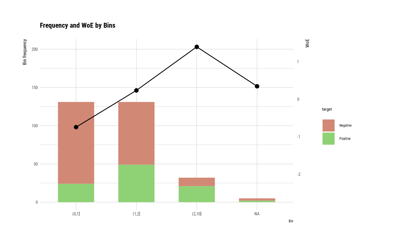
plot(perf)


# Diagnose performance binned variable without NA
perf <- performance_bin(heartfailure2$death_event_2, heartfailure2$creatinine_bin, na.rm = TRUE) 
perf
#>      Bin CntRec CntPos CntNeg CntCumPos CntCumNeg RatePos RateNeg RateCumPos
#> 1  (0,1]    131     24    107        24       107 0.25532   0.535    0.25532
#> 2  (1,2]    131     49     82        73       189 0.52128   0.410    0.77660
#> 3 (2,10]     32     21     11        94       200 0.22340   0.055    1.00000
#> 4  Total    294     94    200        NA        NA 1.00000   1.000         NA
#>   RateCumNeg    Odds   LnOdds      WoE      IV     JSD     AUC
#> 1      0.535 0.22430 -1.49478 -0.73975 0.20689 0.02529 0.06830
#> 2      0.945 0.59756 -0.51490  0.24012 0.02672 0.00333 0.21154
#> 3      1.000 1.90909  0.64663  1.40165 0.23604 0.02731 0.04886
#> 4         NA 0.47000 -0.75502       NA 0.46966 0.05592 0.32870
summary(perf)
#> ── Binning Table ──────────────────────── Several Metrics ── 
#>      Bin CntRec CntPos CntNeg RatePos RateNeg    Odds      WoE      IV     JSD
#> 1  (0,1]    131     24    107 0.25532   0.535 0.22430 -0.73975 0.20689 0.02529
#> 2  (1,2]    131     49     82 0.52128   0.410 0.59756  0.24012 0.02672 0.00333
#> 3 (2,10]     32     21     11 0.22340   0.055 1.90909  1.40165 0.23604 0.02731
#> 4  Total    294     94    200 1.00000   1.000 0.47000       NA 0.46966 0.05592
#>       AUC
#> 1 0.06830
#> 2 0.21154
#> 3 0.04886
#> 4 0.32870
#> 
#> ── General Metrics ───────────────────────────────────────── 
#> • Gini index                       :  -0.34261
#> • IV (Jeffrey)                     :  0.46966
#> • JS (Jensen-Shannon) Divergence   :  0.05592
#> • Kolmogorov-Smirnov Statistics    :  0.27968
#> • HHI (Herfindahl-Hirschman Index) :  0.40893
#> • HHI (normalized)                 :  0.11339
#> • Cramer's V                       :  0.31765 
#> 
#> ── Significance Tests ──────────────────── Chisquare Test ── 
#>   Bin A  Bin B statistics     p_value
#> 1 (0,1]  (1,2]   11.86852 0.000570907
#> 2 (1,2] (2,10]    8.35901 0.003837797
#> 

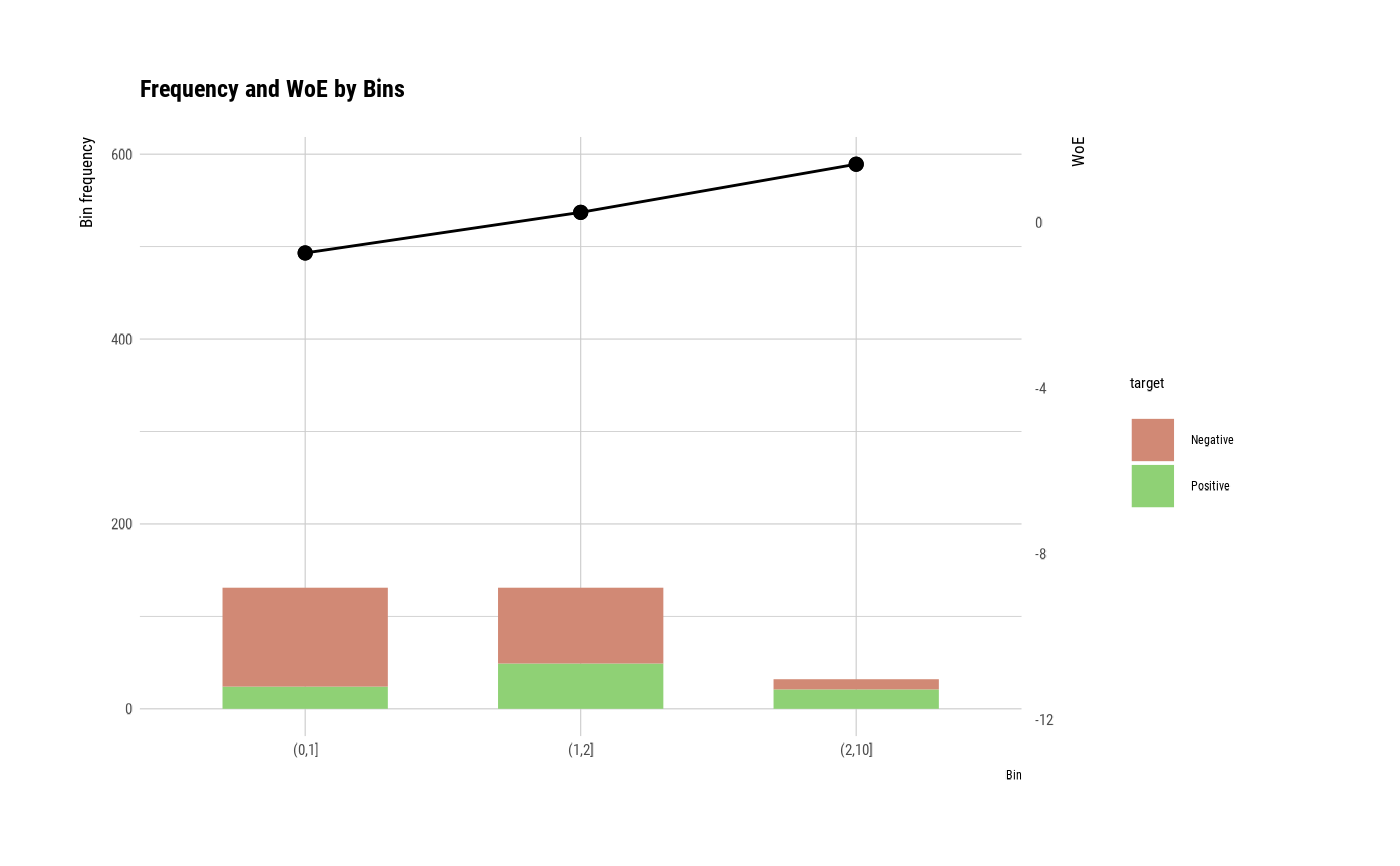
plot(perf)

# }

Arguments

Value

Details

See also

Examples