Visualize Performance for an

It generates plots for understand frequency, WoE by bins using performance_bin.

# S3 method for performance_bin
plot(x, typographic = TRUE, base_family = NULL, ...)

Arguments

x	an object of class "performance_bin", usually, a result of a call to performance_bin().
typographic	logical. Whether to apply focuses on typographic elements to ggplot2 visualization. The default is TRUE. if TRUE provides a base theme that focuses on typographic elements using hrbrthemes package.
base_family	character. The name of the base font family to use for the visualization. If not specified, the font defined in dlookr is applied. (See details)
...	further arguments to be passed from or to other methods.

Details

The base_family is selected from "Roboto Condensed", "Liberation Sans Narrow", "NanumSquare", "Noto Sans Korean". If you want to use a different font, use it after loading the Google font with import_google_font().

Examples

# \donttest{
# Generate data for the example
heartfailure2 <- heartfailure

set.seed(123)
heartfailure2[sample(seq(NROW(heartfailure2)), 5), "creatinine"] <- NA

# Change the target variable to 0(negative) and 1(positive).
heartfailure2$death_event_2 <- ifelse(heartfailure2$death_event %in% "Yes", 1, 0)

# Binnig from creatinine to platelets_bin.
breaks <- c(0,  1,  2, 10)
heartfailure2$creatinine_bin <- cut(heartfailure2$creatinine, breaks)

# Diagnose performance binned variable
perf <- performance_bin(heartfailure2$death_event_2, heartfailure2$creatinine_bin)
perf
#>      Bin CntRec CntPos CntNeg CntCumPos CntCumNeg RatePos RateNeg RateCumPos
#> 1  (0,1]    128     24    104        24       104 0.25000 0.51232    0.25000
#> 2  (1,2]    132     51     81        75       185 0.53125 0.39901    0.78125
#> 3 (2,10]     34     21     13        96       198 0.21875 0.06404    1.00000
#> 4   <NA>      5      0      5        96       203 0.00000 0.02463    1.00000
#> 5  Total    299     96    203        NA        NA 1.00000 1.00000         NA
#>   RateCumNeg    Odds   LnOdds      WoE      IV     JSD     AUC
#> 1    0.51232 0.23077 -1.46634 -0.71748 0.18821 0.02303 0.06404
#> 2    0.91133 0.62963 -0.46262  0.28623 0.03785 0.00472 0.20574
#> 3    0.97537 1.61538  0.47957  1.22843 0.19005 0.02237 0.05704
#> 4    1.00000 0.00000     -Inf       NA      NA      NA 0.02463
#> 5         NA 0.47291 -0.74886       NA      NA      NA 0.35145
summary(perf)
#> ── Binning Table ──────────────────────── Several Metrics ── 
#>      Bin CntRec CntPos CntNeg RatePos RateNeg    Odds      WoE      IV     JSD
#> 1  (0,1]    128     24    104 0.25000 0.51232 0.23077 -0.71748 0.18821 0.02303
#> 2  (1,2]    132     51     81 0.53125 0.39901 0.62963  0.28623 0.03785 0.00472
#> 3 (2,10]     34     21     13 0.21875 0.06404 1.61538  1.22843 0.19005 0.02237
#> 4   <NA>      5      0      5 0.00000 0.02463 0.00000       NA      NA      NA
#> 5  Total    299     96    203 1.00000 1.00000 0.47291       NA      NA      NA
#>       AUC
#> 1 0.06404
#> 2 0.20574
#> 3 0.05704
#> 4 0.02463
#> 5 0.35145
#> 
#> ── General Metrics ───────────────────────────────────────── 
#> • Gini index                       :  -0.29711
#> • IV (Jeffrey)                     :  NA
#> • JS (Jensen-Shannon) Divergence   :  NA
#> • Kolmogorov-Smirnov Statistics    :  0.26232
#> • HHI (Herfindahl-Hirschman Index) :  0.39137
#> • HHI (normalized)                 :  0.1885
#> • Cramer's V                       :  0.30024 
#> 
#> ── Significance Tests ──────────────────── Chisquare Test ── 
#>   Bin A  Bin B statistics      p_value
#> 1 (0,1]  (1,2]  12.520885 0.0004024283
#> 2 (1,2] (2,10]   5.888296 0.0152418462
#> 

plot(perf)
#> Warning: Removed 2 rows containing missing values (geom_point).
#> Warning: Removed 2 row(s) containing missing values (geom_path).

# Diagnose performance binned variable without NA
perf <- performance_bin(heartfailure2$death_event_2, heartfailure2$creatinine_bin, na.rm = TRUE)
perf
#>      Bin CntRec CntPos CntNeg CntCumPos CntCumNeg RatePos RateNeg RateCumPos
#> 1  (0,1]    128     24    104        24       104 0.25000 0.52525    0.25000
#> 2  (1,2]    132     51     81        75       185 0.53125 0.40909    0.78125
#> 3 (2,10]     34     21     13        96       198 0.21875 0.06566    1.00000
#> 4  Total    294     96    198        NA        NA 1.00000 1.00000         NA
#>   RateCumNeg    Odds   LnOdds      WoE      IV     JSD     AUC
#> 1    0.52525 0.23077 -1.46634 -0.74242 0.20435 0.02497 0.06566
#> 2    0.93434 0.62963 -0.46262  0.26130 0.03192 0.00398 0.21094
#> 3    1.00000 1.61538  0.47957  1.20349 0.18425 0.02173 0.05848
#> 4         NA 0.48485 -0.72392       NA 0.42052 0.05069 0.33507
summary(perf)
#> ── Binning Table ──────────────────────── Several Metrics ── 
#>      Bin CntRec CntPos CntNeg RatePos RateNeg    Odds      WoE      IV     JSD
#> 1  (0,1]    128     24    104 0.25000 0.52525 0.23077 -0.74242 0.20435 0.02497
#> 2  (1,2]    132     51     81 0.53125 0.40909 0.62963  0.26130 0.03192 0.00398
#> 3 (2,10]     34     21     13 0.21875 0.06566 1.61538  1.20349 0.18425 0.02173
#> 4  Total    294     96    198 1.00000 1.00000 0.48485       NA 0.42052 0.05069
#>       AUC
#> 1 0.06566
#> 2 0.21094
#> 3 0.05848
#> 4 0.33507
#> 
#> ── General Metrics ───────────────────────────────────────── 
#> • Gini index                       :  -0.32986
#> • IV (Jeffrey)                     :  0.42052
#> • JS (Jensen-Shannon) Divergence   :  0.05069
#> • Kolmogorov-Smirnov Statistics    :  0.27525
#> • HHI (Herfindahl-Hirschman Index) :  0.40451
#> • HHI (normalized)                 :  0.10676
#> • Cramer's V                       :  0.30024 
#> 
#> ── Significance Tests ──────────────────── Chisquare Test ── 
#>   Bin A  Bin B statistics      p_value
#> 1 (0,1]  (1,2]  12.520885 0.0004024283
#> 2 (1,2] (2,10]   5.888296 0.0152418462
#> 

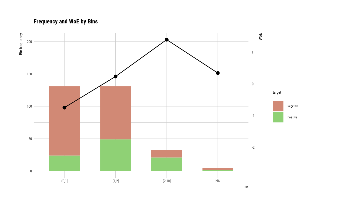
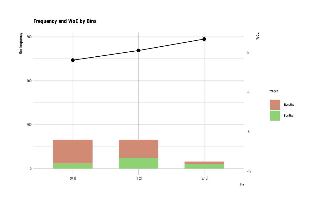
plot(perf)
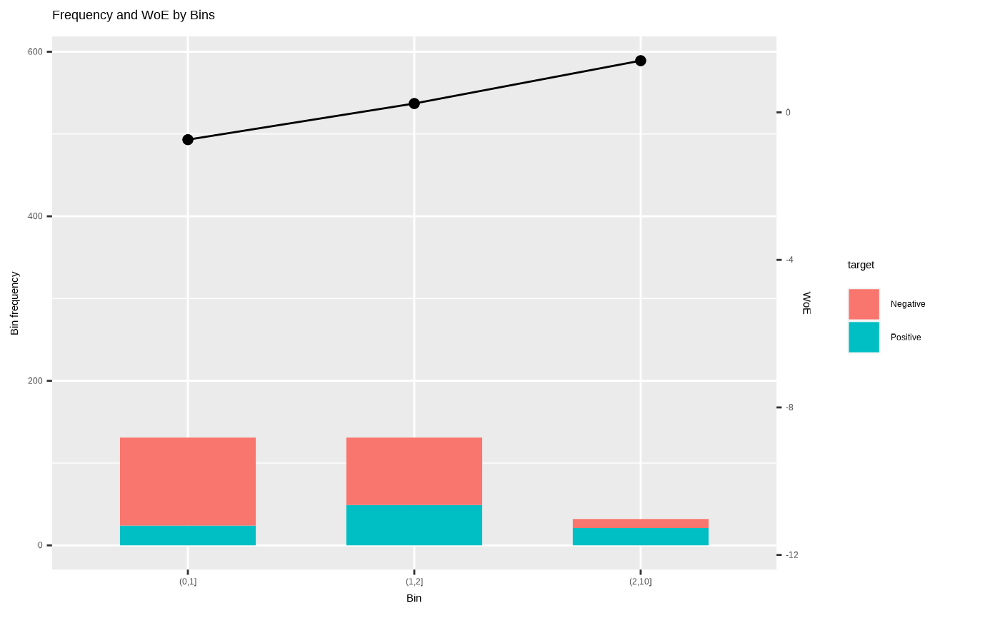
plot(perf, typographic = FALSE)
# }

Visualize Performance for an "performance_bin" Object

Arguments

Details

See also

Examples