Visualize mosaics plot by attribute of compare_category class.

# S3 method for compare_category
plot(
  x,
  prompt = FALSE,
  na.rm = FALSE,
  typographic = TRUE,
  base_family = NULL,
  ...
)

Arguments

x

an object of class "compare_category", usually, a result of a call to compare_category().

prompt

logical. The default value is FALSE. If there are multiple visualizations to be output, if this argument value is TRUE, a prompt is output each time.

na.rm

logical. Specifies whether to include NA when plotting mosaics plot. The default is FALSE, so plot NA.

typographic

logical. Whether to apply focuses on typographic elements to ggplot2 visualization. The default is TRUE. if TRUE provides a base theme that focuses on typographic elements using hrbrthemes package.

base_family

character. The name of the base font family to use for the visualization. If not specified, the font defined in dlookr is applied. (See details)

...

arguments to be passed to methods, such as graphical parameters (see par). However, it only support las parameter. las is numeric in 0,1; the style of axis labels.

  • 0 : always parallel to the axis [default],

  • 1 : always horizontal to the axis,

Details

The base_family is selected from "Roboto Condensed", "Liberation Sans Narrow", "NanumSquare", "Noto Sans Korean". If you want to use a different font, use it after loading the Google font with import_google_font().

See also

Examples

# \donttest{ # 
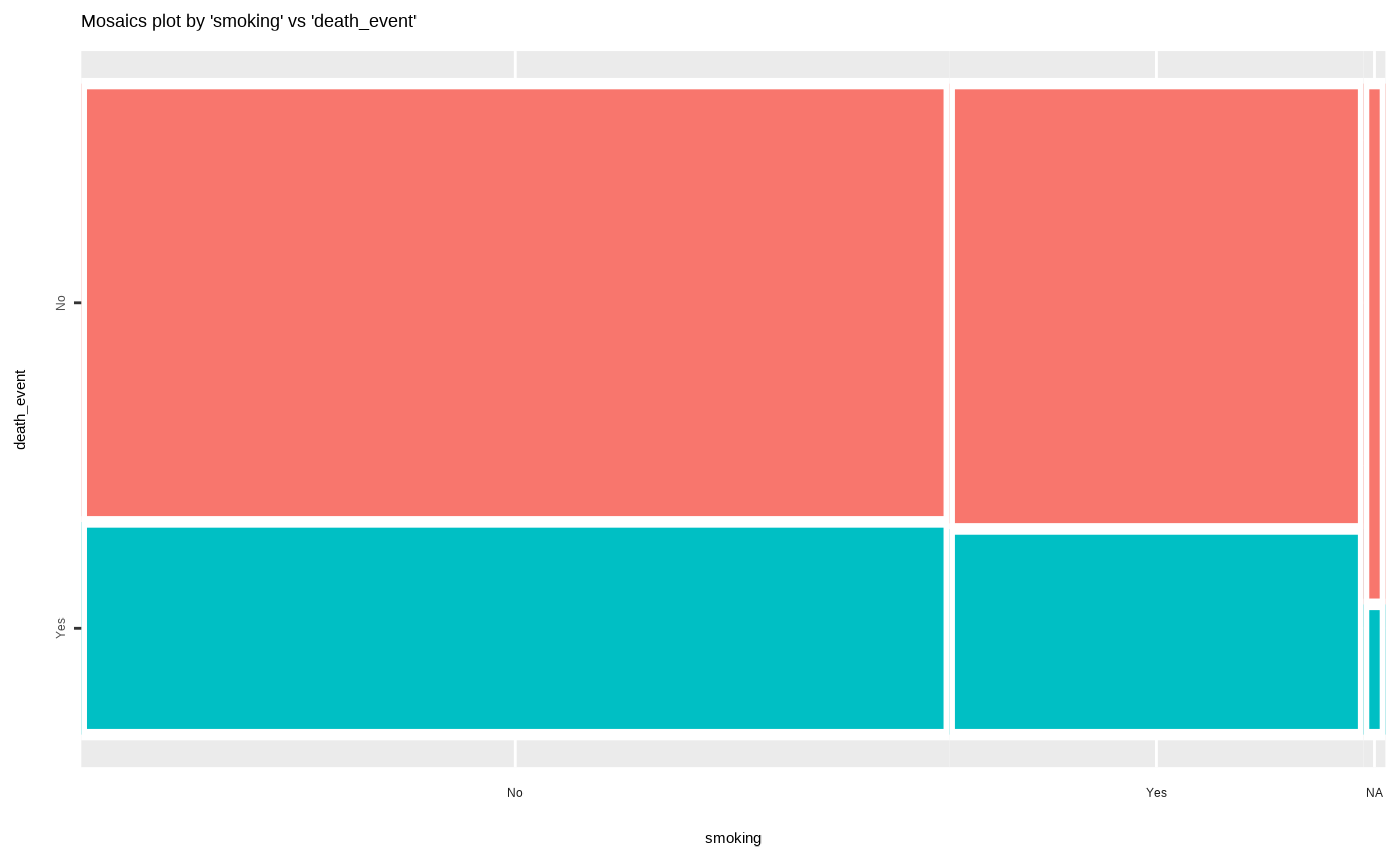
Generate data for the example heartfailure2 <- heartfailure heartfailure2[sample(seq(NROW(heartfailure2)), 5), "smoking"] <- NA library(dplyr) # Compare the all categorical variables all_var <- compare_category(heartfailure2) # Print compare_numeric class objects all_var
#> $`anaemia vs diabetes` #> # A tibble: 4 x 6 #> anaemia diabetes n rate var1_rate var2_rate #> <fct> <fct> <int> <dbl> <dbl> <dbl> #> 1 No No 98 0.328 0.576 0.563 #> 2 No Yes 72 0.241 0.424 0.576 #> 3 Yes No 76 0.254 0.589 0.437 #> 4 Yes Yes 53 0.177 0.411 0.424 #> #> $`anaemia vs hblood_pressure` #> # A tibble: 4 x 6 #> anaemia hblood_pressure n rate var1_rate var2_rate #> <fct> <fct> <int> <dbl> <dbl> <dbl> #> 1 No No 113 0.378 0.665 0.582 #> 2 No Yes 57 0.191 0.335 0.543 #> 3 Yes No 81 0.271 0.628 0.418 #> 4 Yes Yes 48 0.161 0.372 0.457 #> #> $`anaemia vs sex` #> # A tibble: 4 x 6 #> anaemia sex n rate var1_rate var2_rate #> <fct> <fct> <int> <dbl> <dbl> <dbl> #> 1 No Female 53 0.177 0.312 0.505 #> 2 No Male 117 0.391 0.688 0.603 #> 3 Yes Female 52 0.174 0.403 0.495 #> 4 Yes Male 77 0.258 0.597 0.397 #> #> $`anaemia vs smoking` #> # A tibble: 5 x 6 #> anaemia smoking n rate var1_rate var2_rate #> <fct> <fct> <int> <dbl> <dbl> <dbl> #> 1 No No 108 0.361 0.635 0.543 #> 2 No Yes 62 0.207 0.365 0.653 #> 3 Yes No 91 0.304 0.705 0.457 #> 4 Yes Yes 33 0.110 0.256 0.347 #> 5 Yes NA 5 0.0167 0.0388 1 #> #> $`anaemia vs death_event` #> # A tibble: 4 x 6 #> anaemia death_event n rate var1_rate var2_rate #> <fct> <fct> <int> <dbl> <dbl> <dbl> #> 1 No No 120 0.401 0.706 0.591 #> 2 No Yes 50 0.167 0.294 0.521 #> 3 Yes No 83 0.278 0.643 0.409 #> 4 Yes Yes 46 0.154 0.357 0.479 #> #> $`diabetes vs hblood_pressure` #> # A tibble: 4 x 6 #> diabetes hblood_pressure n rate var1_rate var2_rate #> <fct> <fct> <int> <dbl> <dbl> <dbl> #> 1 No No 112 0.375 0.644 0.577 #> 2 No Yes 62 0.207 0.356 0.590 #> 3 Yes No 82 0.274 0.656 0.423 #> 4 Yes Yes 43 0.144 0.344 0.410 #> #> $`diabetes vs sex` #> # A tibble: 4 x 6 #> diabetes sex n rate var1_rate var2_rate #> <fct> <fct> <int> <dbl> <dbl> <dbl> #> 1 No Female 50 0.167 0.287 0.476 #> 2 No Male 124 0.415 0.713 0.639 #> 3 Yes Female 55 0.184 0.44 0.524 #> 4 Yes Male 70 0.234 0.56 0.361 #> #> $`diabetes vs smoking` #> # A tibble: 6 x 6 #> diabetes smoking n rate var1_rate var2_rate #> <fct> <fct> <int> <dbl> <dbl> <dbl> #> 1 No No 106 0.355 0.609 0.533 #> 2 No Yes 65 0.217 0.374 0.684 #> 3 No NA 3 0.0100 0.0172 0.6 #> 4 Yes No 93 0.311 0.744 0.467 #> 5 Yes Yes 30 0.100 0.24 0.316 #> 6 Yes NA 2 0.00669 0.016 0.4 #> #> $`diabetes vs death_event` #> # A tibble: 4 x 6 #> diabetes death_event n rate var1_rate var2_rate #> <fct> <fct> <int> <dbl> <dbl> <dbl> #> 1 No No 118 0.395 0.678 0.581 #> 2 No Yes 56 0.187 0.322 0.583 #> 3 Yes No 85 0.284 0.68 0.419 #> 4 Yes Yes 40 0.134 0.32 0.417 #> #> $`hblood_pressure vs sex` #> # A tibble: 4 x 6 #> hblood_pressure sex n rate var1_rate var2_rate #> <fct> <fct> <int> <dbl> <dbl> <dbl> #> 1 No Female 61 0.204 0.314 0.581 #> 2 No Male 133 0.445 0.686 0.686 #> 3 Yes Female 44 0.147 0.419 0.419 #> 4 Yes Male 61 0.204 0.581 0.314 #> #> $`hblood_pressure vs smoking` #> # A tibble: 6 x 6 #> hblood_pressure smoking n rate var1_rate var2_rate #> <fct> <fct> <int> <dbl> <dbl> <dbl> #> 1 No No 126 0.421 0.649 0.633 #> 2 No Yes 66 0.221 0.340 0.695 #> 3 No NA 2 0.00669 0.0103 0.4 #> 4 Yes No 73 0.244 0.695 0.367 #> 5 Yes Yes 29 0.0970 0.276 0.305 #> 6 Yes NA 3 0.0100 0.0286 0.6 #> #> $`hblood_pressure vs death_event` #> # A tibble: 4 x 6 #> hblood_pressure death_event n rate var1_rate var2_rate #> <fct> <fct> <int> <dbl> <dbl> <dbl> #> 1 No No 137 0.458 0.706 0.675 #> 2 No Yes 57 0.191 0.294 0.594 #> 3 Yes No 66 0.221 0.629 0.325 #> 4 Yes Yes 39 0.130 0.371 0.406 #> #> $`sex vs smoking` #> # A tibble: 6 x 6 #> sex smoking n rate var1_rate var2_rate #> <fct> <fct> <int> <dbl> <dbl> <dbl> #> 1 Female No 99 0.331 0.943 0.497 #> 2 Female Yes 4 0.0134 0.0381 0.0421 #> 3 Female NA 2 0.00669 0.0190 0.4 #> 4 Male No 100 0.334 0.515 0.503 #> 5 Male Yes 91 0.304 0.469 0.958 #> 6 Male NA 3 0.0100 0.0155 0.6 #> #> $`sex vs death_event` #> # A tibble: 4 x 6 #> sex death_event n rate var1_rate var2_rate #> <fct> <fct> <int> <dbl> <dbl> <dbl> #> 1 Female No 71 0.237 0.676 0.350 #> 2 Female Yes 34 0.114 0.324 0.354 #> 3 Male No 132 0.441 0.680 0.650 #> 4 Male Yes 62 0.207 0.320 0.646 #> #> $`smoking vs death_event` #> # A tibble: 6 x 6 #> smoking death_event n rate var1_rate var2_rate #> <fct> <fct> <int> <dbl> <dbl> <dbl> #> 1 No No 134 0.448 0.673 0.660 #> 2 No Yes 65 0.217 0.327 0.677 #> 3 Yes No 65 0.217 0.684 0.320 #> 4 Yes Yes 30 0.100 0.316 0.312 #> 5 NA No 4 0.0134 0.8 0.0197 #> 6 NA Yes 1 0.00334 0.2 0.0104 #>
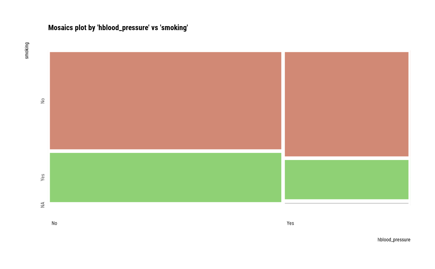
# Compare the two categorical variables two_var <- compare_category(heartfailure2, smoking, death_event) # Print compare_category class objects two_var
#> $`smoking vs death_event` #> # A tibble: 6 x 6 #> smoking death_event n rate var1_rate var2_rate #> <fct> <fct> <int> <dbl> <dbl> <dbl> #> 1 No No 134 0.448 0.673 0.660 #> 2 No Yes 65 0.217 0.327 0.677 #> 3 Yes No 65 0.217 0.684 0.320 #> 4 Yes Yes 30 0.100 0.316 0.312 #> 5 NA No 4 0.0134 0.8 0.0197 #> 6 NA Yes 1 0.00334 0.2 0.0104 #>
# plot all pair of variables # plot(all_var) # plot a pair of variables plot(two_var)
# plot all pair of variables by prompt plot(all_var, prompt = TRUE)
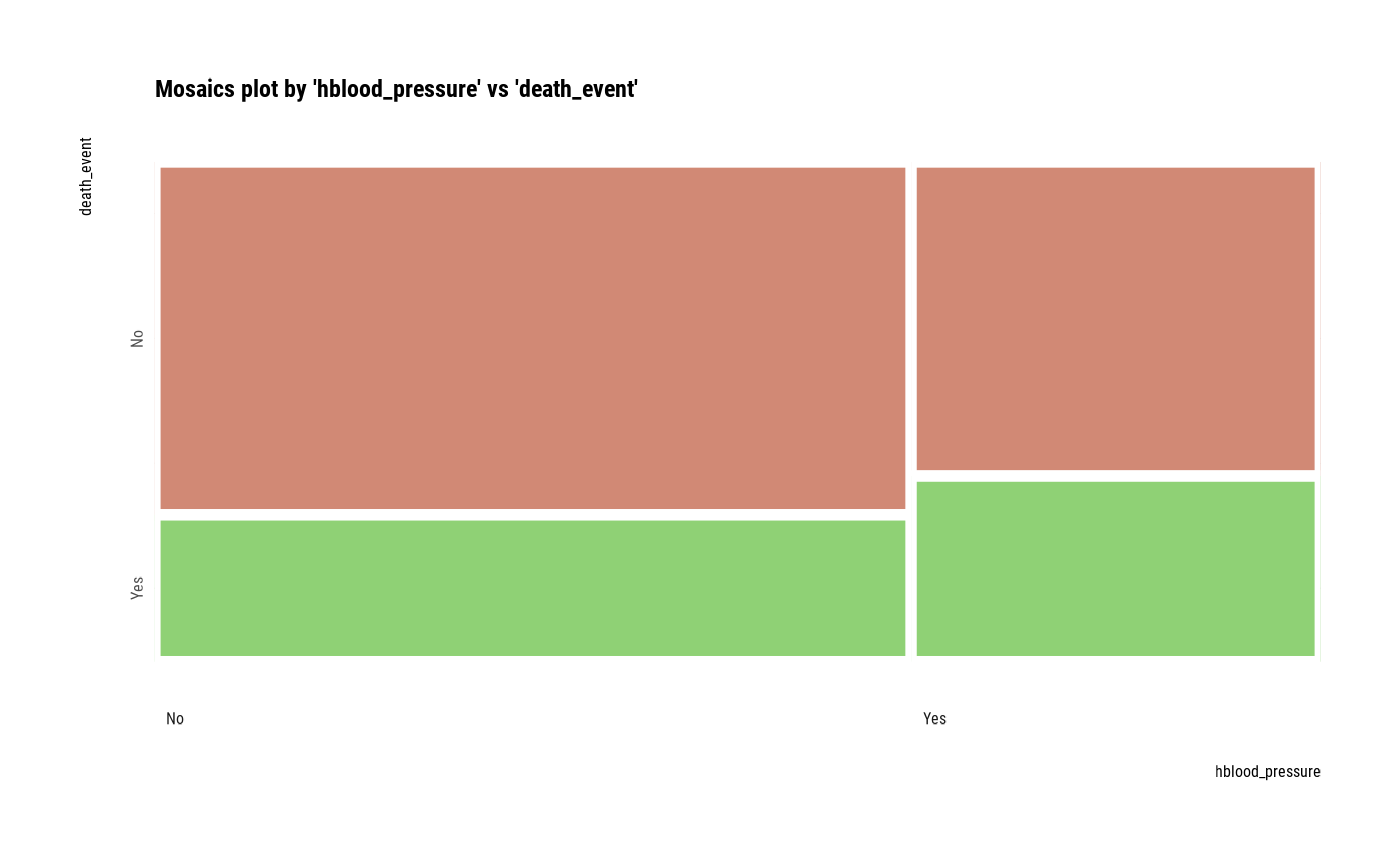
# plot a pair of variables without NA plot(two_var, na.rm = TRUE)
# plot a pair of variables plot(two_var, las = 1)
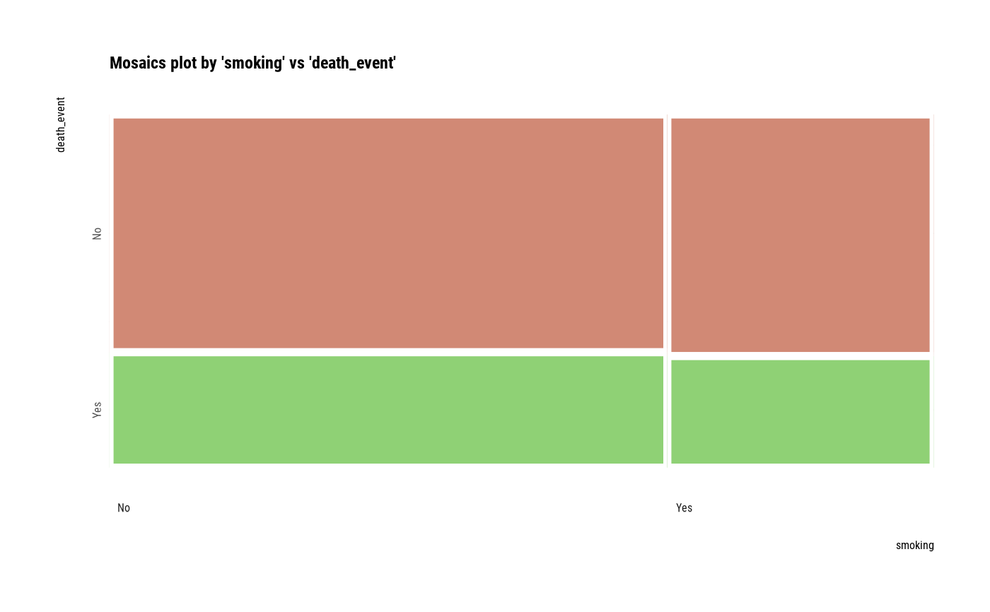
# plot a pair of variables not focuses on typographic elements plot(two_var, typographic = FALSE)
# }