The univar_numeric() calculates statistic of numerical variables that is frequency table
univar_numeric(.data, ...)

# S3 method for class 'data.frame'
univar_numeric(.data, ...)
Arguments
- .data
a data.frame or a
tbl_df.- ...
one or more unquoted expressions separated by commas. You can treat variable names like they are positions. Positive values select variables; negative values to drop variables. These arguments are automatically quoted and evaluated in a context where column names represent column positions. They support unquoting and splicing.
Value
An object of the class as individual variables based list. A component named "statistics" is a tibble object with the following statistics.:
variable : factor. The level of the variable. 'variable' is the name of the variable.
n : number of observations excluding missing values
na : number of missing values
mean : arithmetic average
sd : standard deviation
se_mean : standrd error mean. sd/sqrt(n)
IQR : interquartile range (Q3-Q1)
skewness : skewness
kurtosis : kurtosis
median : median. 50% percentile
Details
univar_numeric() calculates the popular statistics of numerical variables. If a specific variable name is not specified, statistics for all categorical numerical included in the data are calculated. The statistics obtained by univar_numeric() are part of those obtained by describe(). Therefore, it is recommended to use describe() to simply calculate statistics. However, if you want to visualize the distribution of individual variables, you should use univar_numeric().
Attributes of return object
Attributes of compare_category class is as follows.
raw : a data.frame or a
tbl_df. Data containing variables to be compared. Save it for visualization with plot.univar_numeric().variables : character. List of variables selected for calculate statistics.
Examples
# \donttest{
# Calculates the all categorical variables
all_var <- univar_numeric(heartfailure)
# Print univar_numeric class object
all_var
#> $statistics
#> # A tibble: 7 × 10
#> described_variables n na mean sd se_mean IQR skewness
#> <chr> <int> <int> <dbl> <dbl> <dbl> <dbl> <dbl>
#> 1 age 299 0 60.8 11.9 0.688 19 0.424
#> 2 cpk_enzyme 299 0 582. 970. 56.1 466. 4.46
#> 3 ejection_fraction 299 0 38.1 11.8 0.684 15 0.555
#> 4 platelets 299 0 263358. 97804. 5656. 91000 1.46
#> 5 creatinine 299 0 1.39 1.03 0.0598 0.5 4.46
#> 6 sodium 299 0 137. 4.41 0.255 6 -1.05
#> 7 time 299 0 130. 77.6 4.49 130 0.128
#> # ℹ 2 more variables: kurtosis <dbl>, median <dbl>
#>
# Calculates the platelets, sodium variable
univar_numeric(heartfailure, platelets, sodium)
#> $statistics
#> # A tibble: 2 × 10
#> described_variables n na mean sd se_mean IQR skewness kurtosis
#> <chr> <int> <int> <dbl> <dbl> <dbl> <dbl> <dbl> <dbl>
#> 1 platelets 299 0 263358. 9.78e4 5.66e+3 91000 1.46 6.21
#> 2 sodium 299 0 137. 4.41e0 2.55e-1 6 -1.05 4.12
#> # ℹ 1 more variable: median <dbl>
#>
# Summary the all case : Return a invisible copy of an object.
stat <- summary(all_var)
# Summary by returned object
stat
#> # A tibble: 7 × 8
#> described_variables mean sd se_mean IQR skewness kurtosis median
#> <chr> <dbl> <dbl> <dbl> <dbl> <dbl> <dbl> <dbl>
#> 1 age 0.0437 0.626 0.0362 1 0.424 -0.184 0
#> 2 cpk_enzyme 0.713 2.08 0.121 1 4.46 25.1 0
#> 3 ejection_fraction 0.00557 0.789 0.0456 1 0.555 0.0414 0
#> 4 platelets 0.0149 1.07 0.0622 1 1.46 6.21 0
#> 5 creatinine 0.588 2.07 0.120 1 4.46 25.8 0
#> 6 sodium -0.0624 0.735 0.0425 1 -1.05 4.12 0
#> 7 time 0.117 0.597 0.0345 1 0.128 -1.21 0
# Statistics of numerical variables normalized by Min-Max method
summary(all_var, stand = "minmax")
#> # A tibble: 7 × 8
#> described_variables mean sd se_mean IQR skewness kurtosis median
#> <chr> <dbl> <dbl> <dbl> <dbl> <dbl> <dbl> <dbl>
#> 1 age 0.379 0.216 0.0125 0.345 0.424 -0.184 0.364
#> 2 cpk_enzyme 0.0713 0.124 0.00716 0.0594 4.46 25.1 0.0290
#> 3 ejection_fraction 0.365 0.179 0.0104 0.227 0.555 0.0414 0.364
#> 4 platelets 0.289 0.119 0.00686 0.110 1.46 6.21 0.287
#> 5 creatinine 0.100 0.116 0.00672 0.0562 4.46 25.8 0.0674
#> 6 sodium 0.675 0.126 0.00729 0.171 -1.05 4.12 0.686
#> 7 time 0.449 0.276 0.0160 0.463 0.128 -1.21 0.395
# Statistics of numerical variables standardized by Z-score method
summary(all_var, stand = "zscore")
#> # A tibble: 7 × 8
#> described_variables mean sd se_mean IQR skewness kurtosis median
#> <chr> <dbl> <dbl> <dbl> <dbl> <dbl> <dbl> <dbl>
#> 1 age 2.11e-16 1.00 0.0578 1.60 0.424 -0.184 -0.0697
#> 2 cpk_enzyme -2.14e-17 1.00 0.0578 0.480 4.46 25.1 -0.342
#> 3 ejection_fraction 4.75e-17 1.00 0.0578 1.27 0.555 0.0414 -0.00706
#> 4 platelets -1.11e-15 1 0.0578 0.930 1.46 6.21 -0.0139
#> 5 creatinine 4.03e-16 1.00 0.0578 0.483 4.46 25.8 -0.284
#> 6 sodium -8.42e-16 1.00 0.0578 1.36 -1.05 4.12 0.0849
#> 7 time -6.05e-16 1.00 0.0578 1.67 0.128 -1.21 -0.197
# one plot with all variables
plot(all_var)
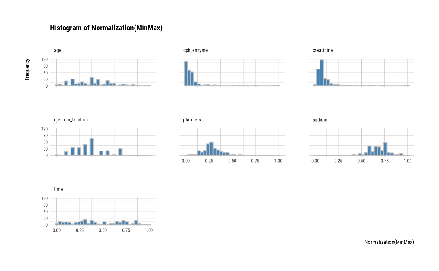
 # one plot with all normalized variables by Min-Max method
plot(all_var, stand = "minmax")
# one plot with all normalized variables by Min-Max method
plot(all_var, stand = "minmax")
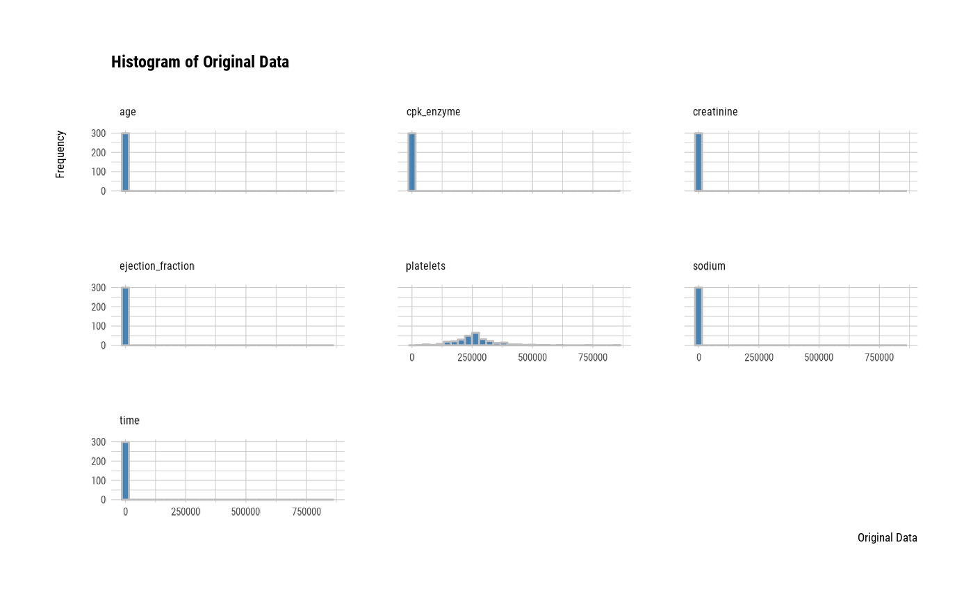
 # one plot with all variables
plot(all_var, stand = "none")
# one plot with all variables
plot(all_var, stand = "none")
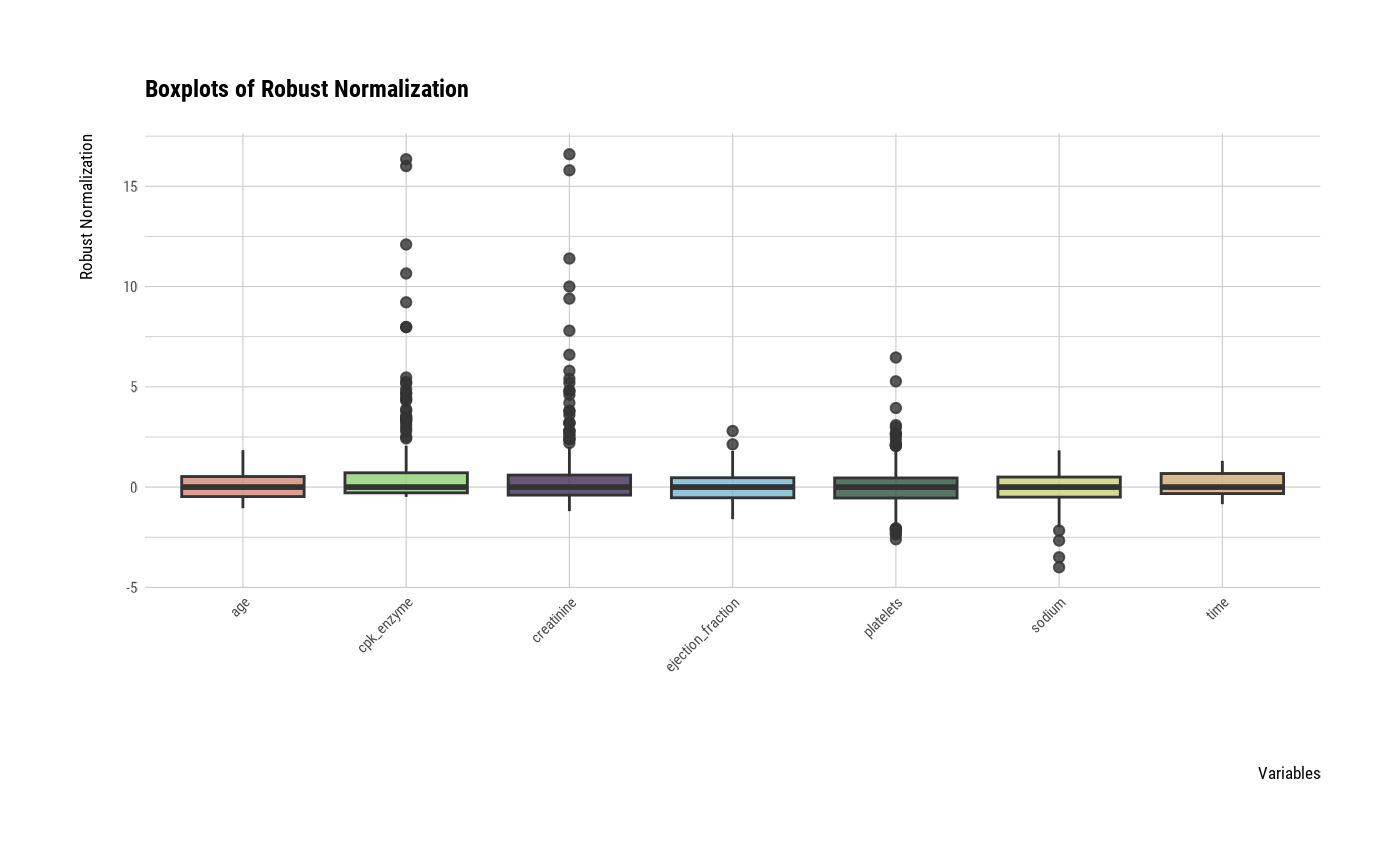
 # one plot with all robust standardized variables
plot(all_var, viz = "boxplot")
# one plot with all robust standardized variables
plot(all_var, viz = "boxplot")
 # one plot with all standardized variables by Z-score method
plot(all_var, viz = "boxplot", stand = "zscore")
# one plot with all standardized variables by Z-score method
plot(all_var, viz = "boxplot", stand = "zscore")
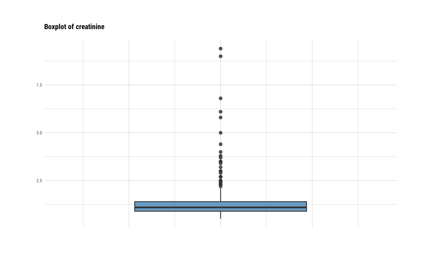
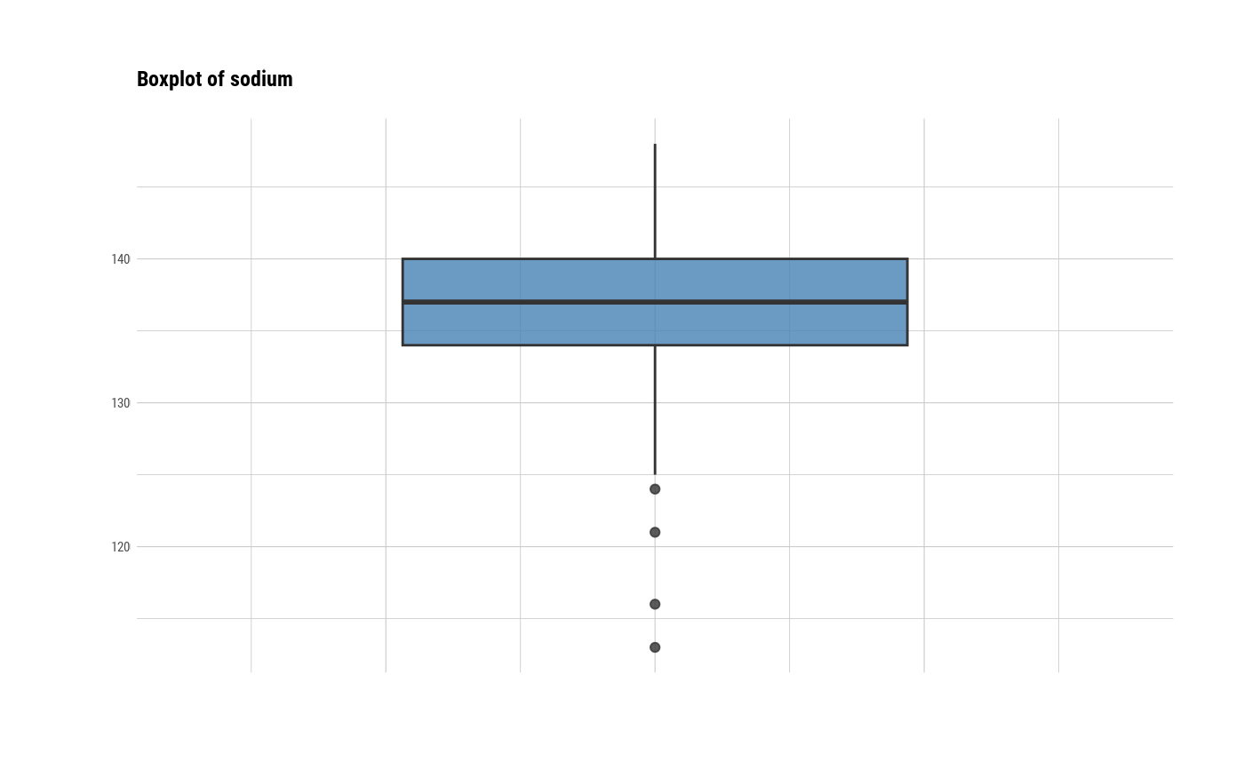
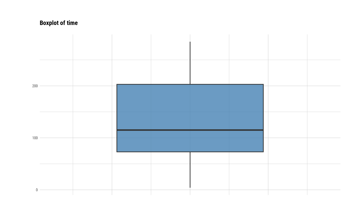
 # individual boxplot by variables
plot(all_var, indiv = TRUE, "boxplot")
# individual boxplot by variables
plot(all_var, indiv = TRUE, "boxplot")
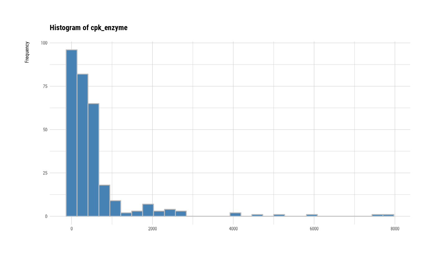
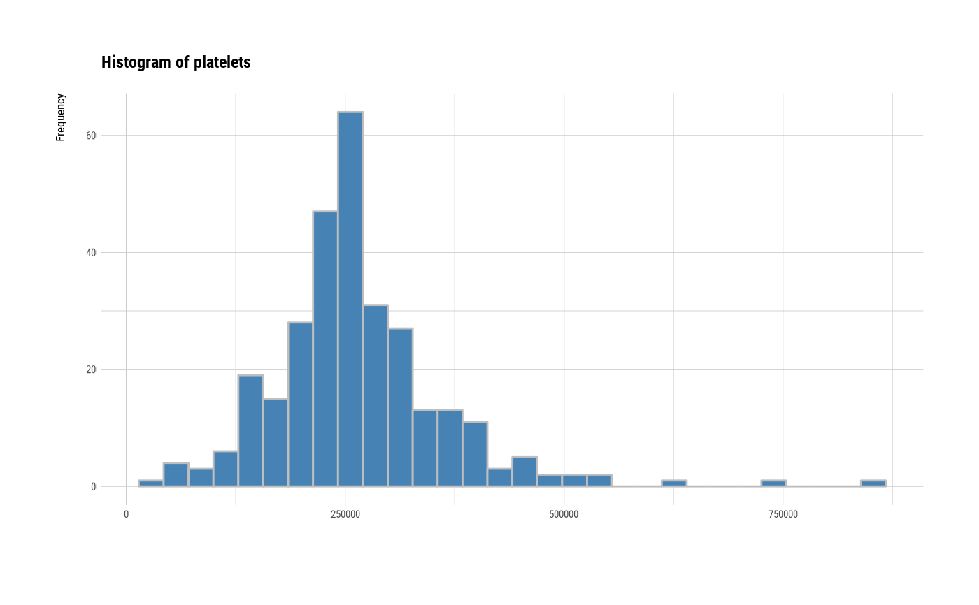
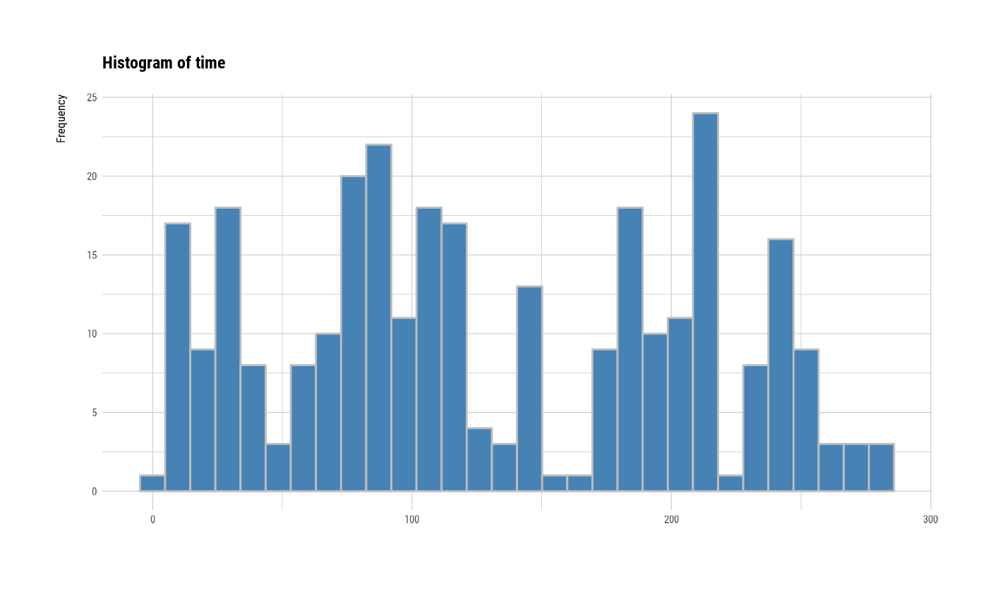
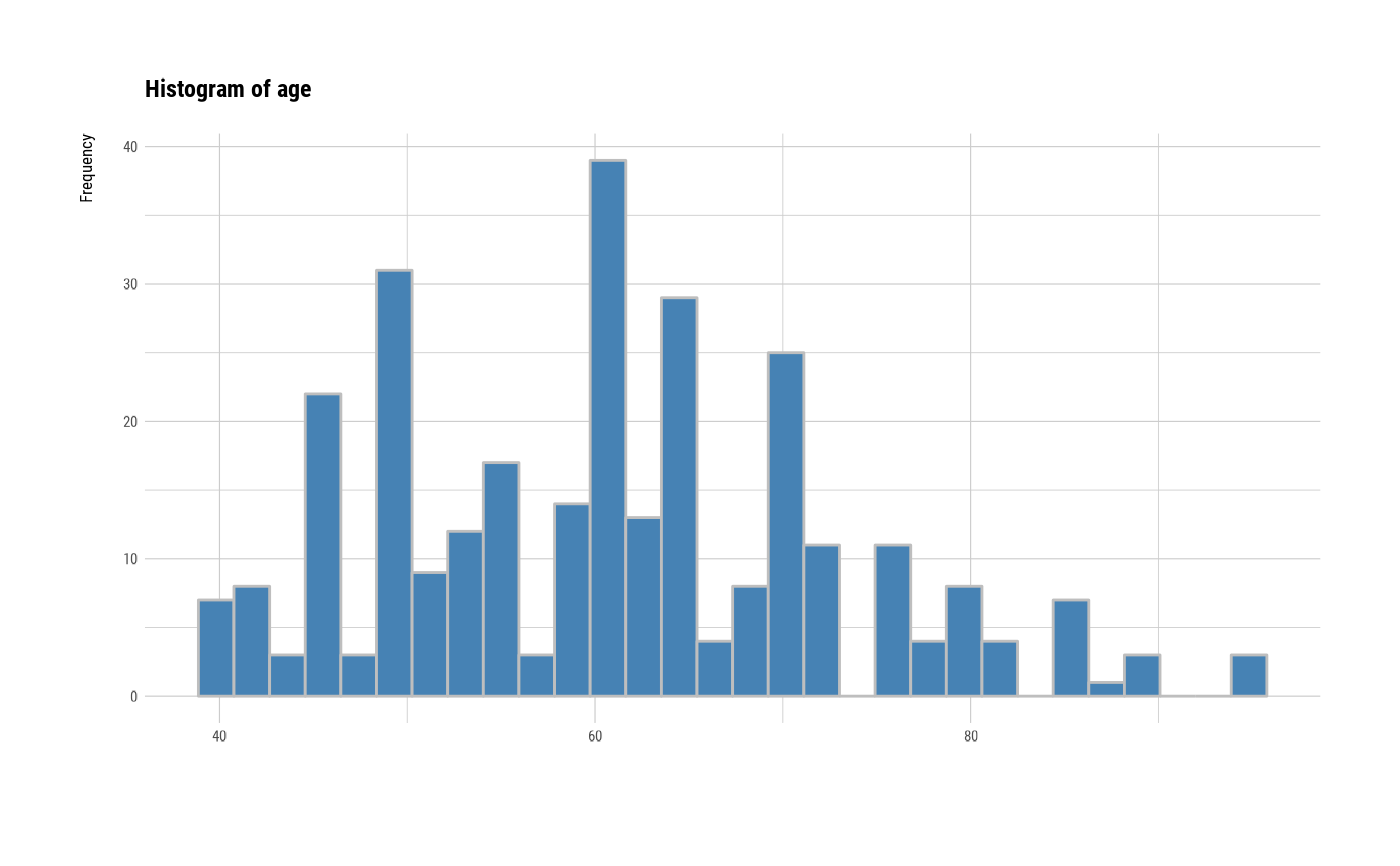
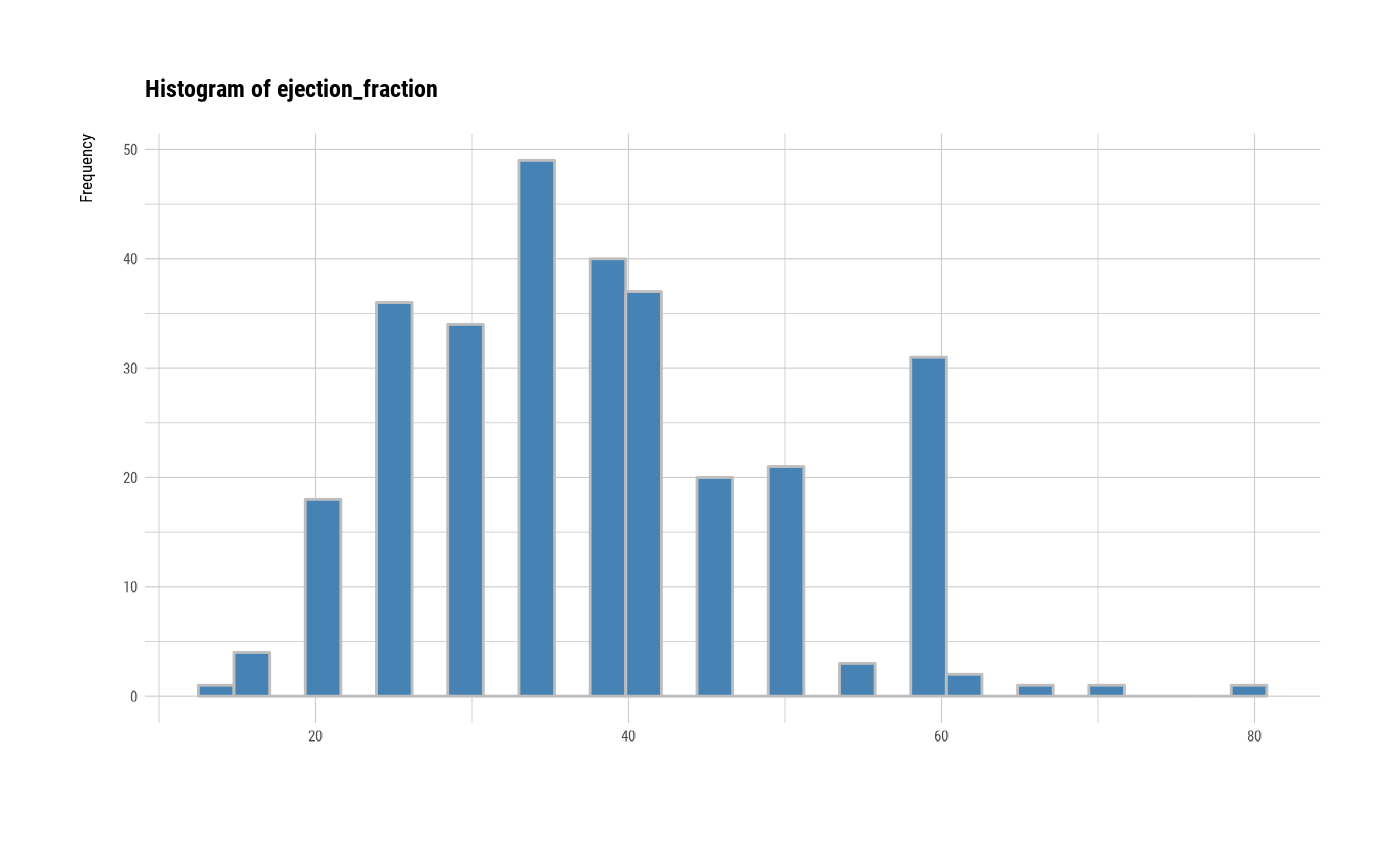
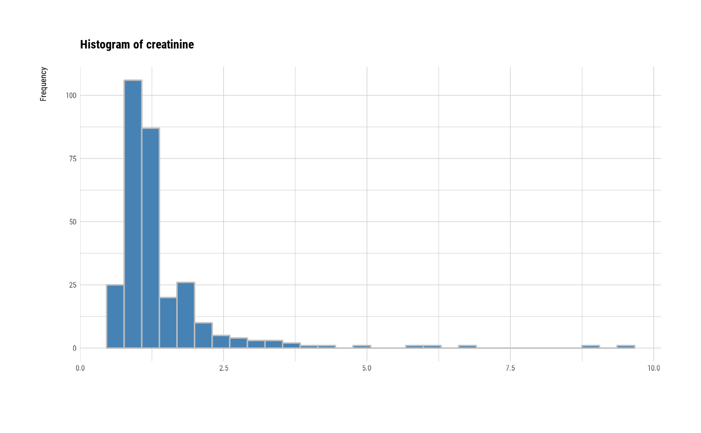
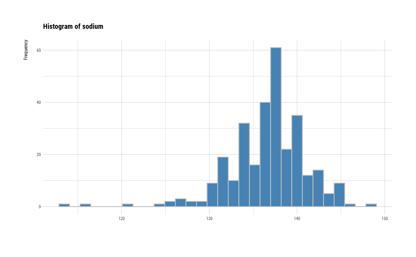
 # individual histogram by variables
plot(all_var, indiv = TRUE, "hist")
# individual histogram by variables
plot(all_var, indiv = TRUE, "hist")


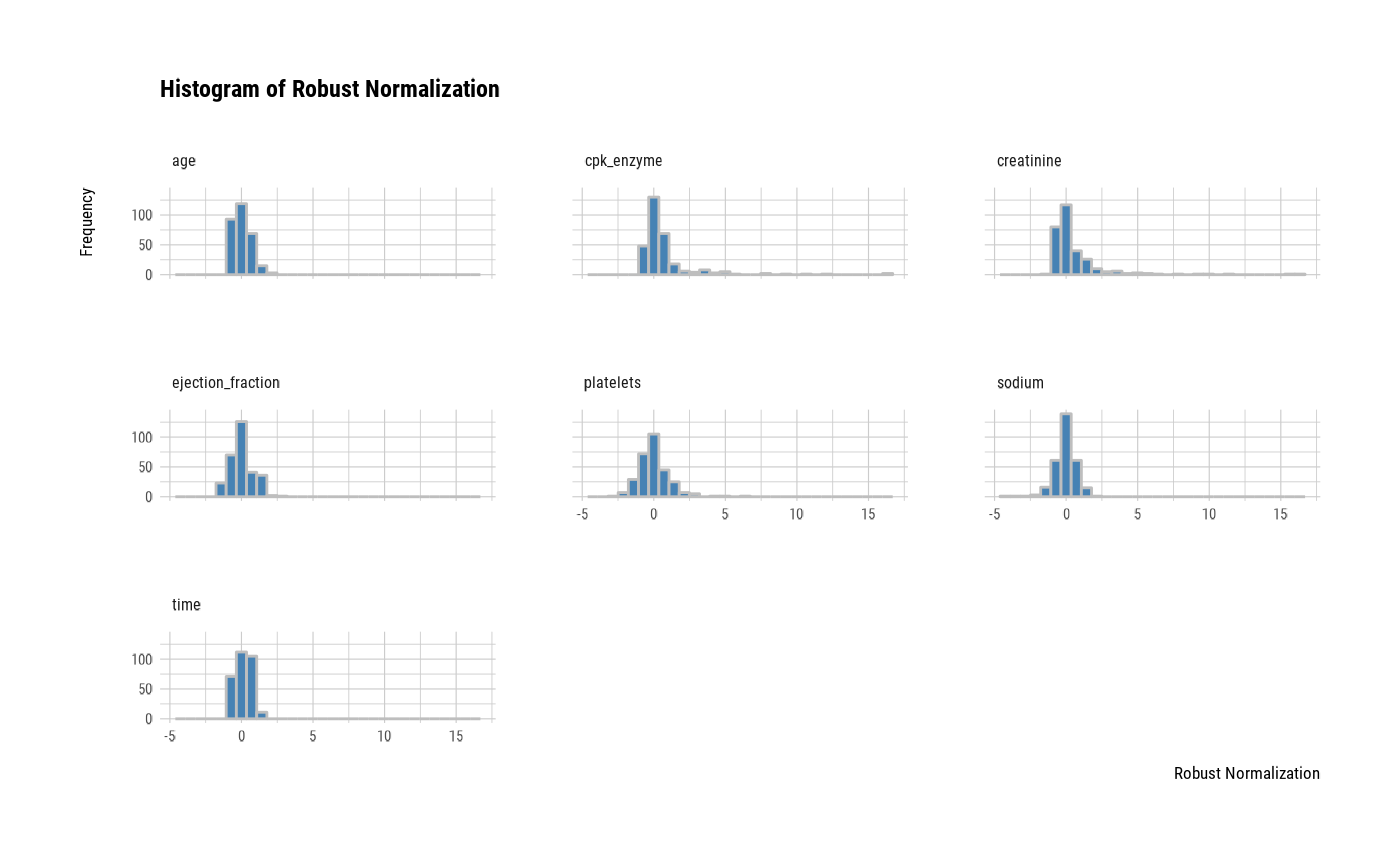
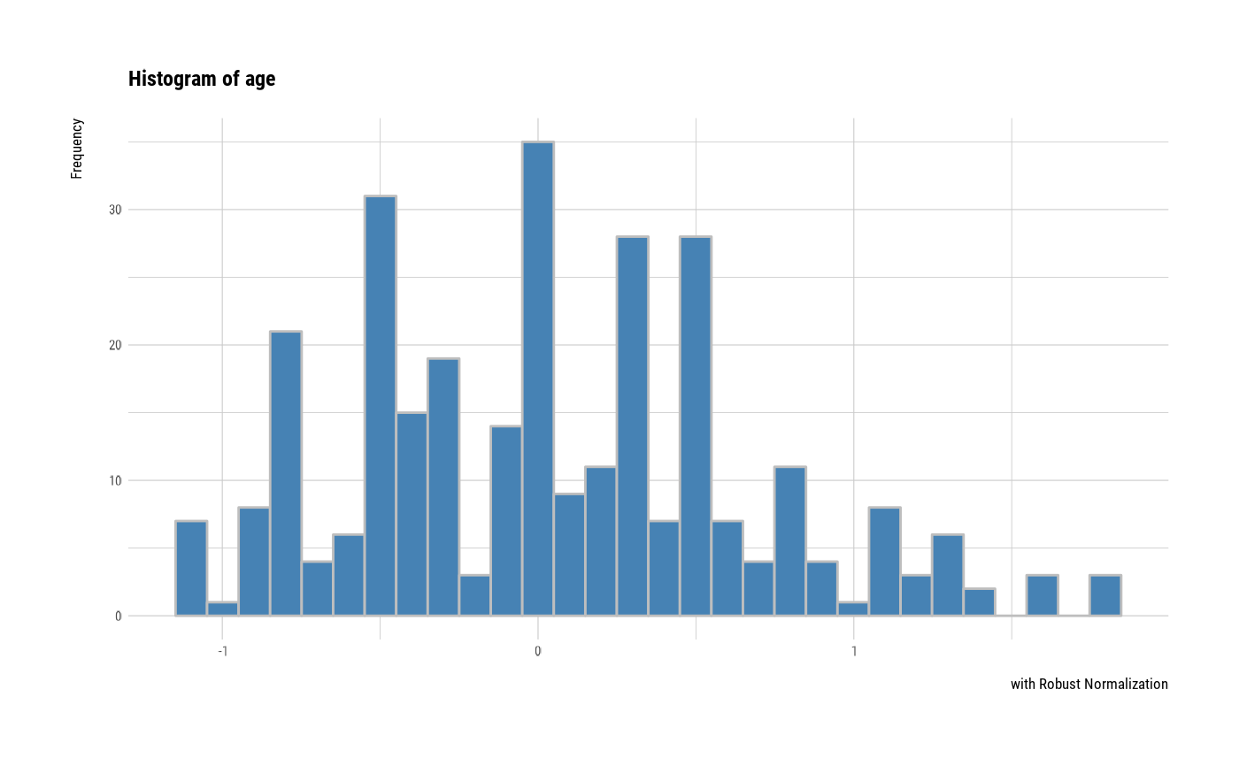
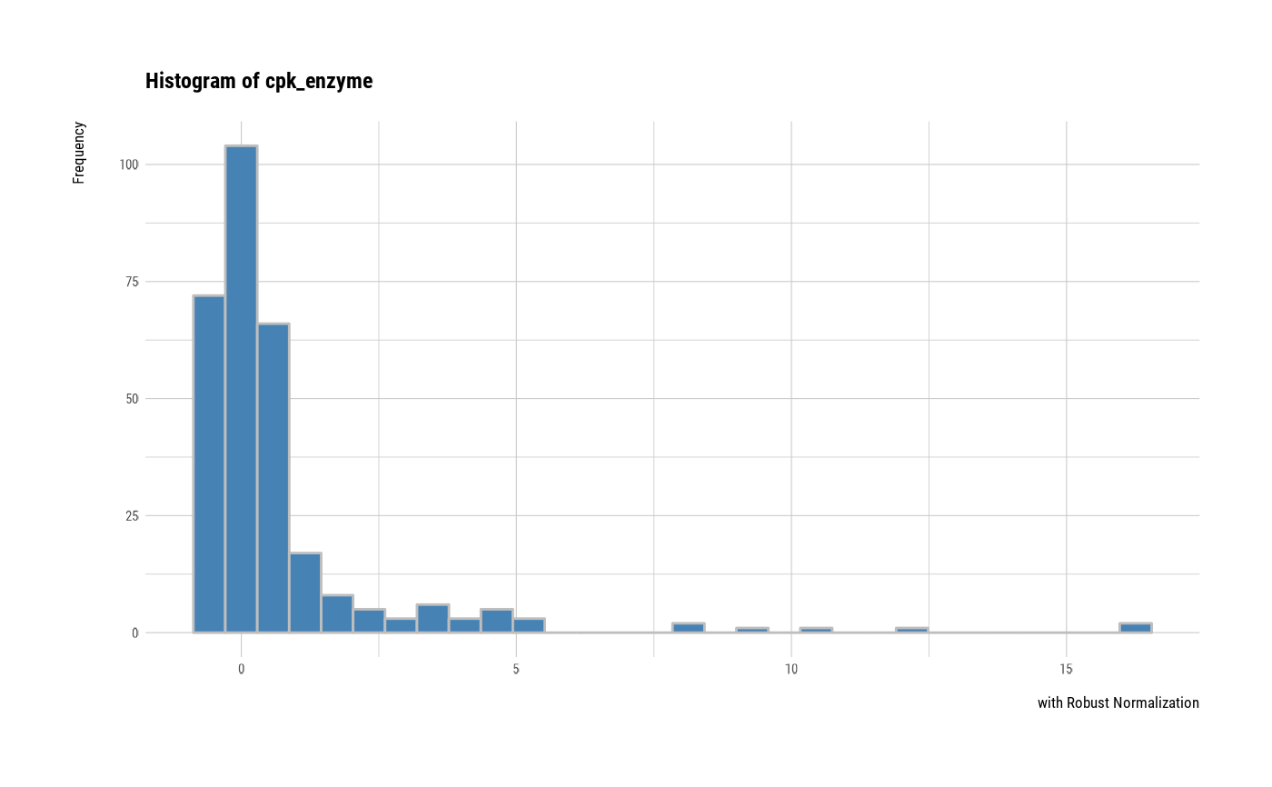
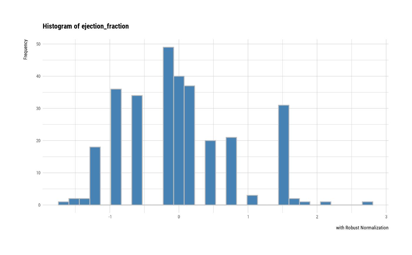
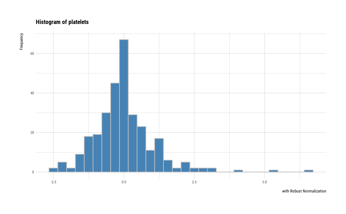
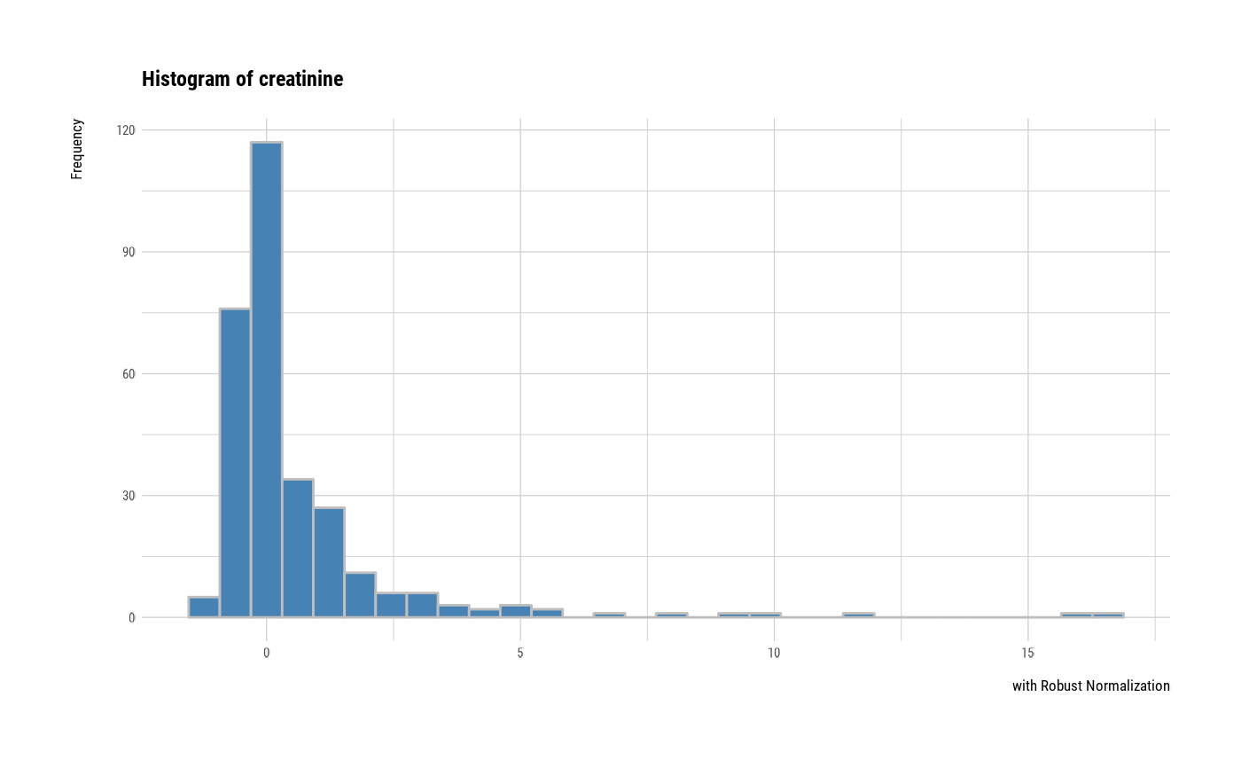
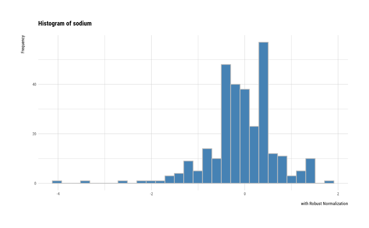
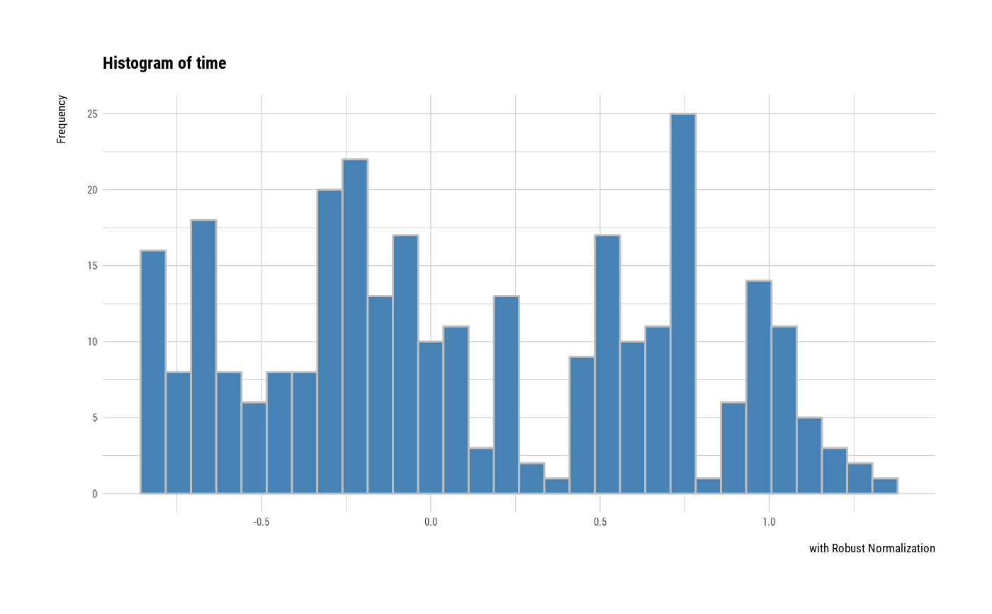
 # individual histogram by robust standardized variable
plot(all_var, indiv = TRUE, "hist", stand = "robust")
# individual histogram by robust standardized variable
plot(all_var, indiv = TRUE, "hist", stand = "robust")
 # plot all variables by prompt
plot(all_var, indiv = TRUE, "hist", prompt = TRUE)
# plot all variables by prompt
plot(all_var, indiv = TRUE, "hist", prompt = TRUE)


 # }
# }